32.1 Introduction
While the main function of food is to provide enjoyment (e.g., flavor, aroma, texture) and nutrition (including energy), some other functionalities (e.g., desired shelf life, improved health benefit, friendly labeling) are also necessary for consumer appeal. One of the trends in food research is to be able to design and produce the food with any desired functionality. To achieve this, many approaches are being taken by different researchers and food manufacturers, with one prevailing approach being to understand and control food structures, especially at the microscopic scale. The study of food microstructures typically involves three aspects – visualization, identification, and quantification – with each requiring the aid of different tools.
Food is a complex and often heterogeneous system. Both fresh (typically dominated with cellular structure) and processed (microscopic domains formed by mixed ingredients) foods contain structures that cannot be directly seen with naked eyes. Human eyes are capable of seeing things down to about 1 μm with proper lighting (compared to ~20 to 50 μm being the diameter of a human hair). Many biological cells are a few micrometers in size, but they are not usually visible to our eyes because good illumination is not always available. They appear big and clear under a regular light microscope. Some good salad dressing emulsions have oil or water droplets well below 1 μm in diameter. Elemental plant fibers have a diameter of only a few nanometers. All these require a higher resolving power microscope such as a scanning electron microscope (SEM).
Determining the morphology of the food with the help of microscopes is only one part of the microstructure elucidation. Identifying the distribution of ingredients with different chemical and physical characteristics gives another insight, and this often requires a chemical imaging tool [e.g., Fourier transform infrared (FTIR), Raman, fluorescence, or confocal laser scanning microscope] or a physical structural tool for understanding molecular arrangement or crystallinity (e.g., x-ray diffractometer).
Modern microscopy and chemical imaging tools allow users to not only determine food morphology and ingredient distribution but also to quantify dimension parameters, concentrations, fractions, and kinetic constants. Using x-ray computed tomography, quantification can be done in 3-D with nondestructive imaging. Microscale interactions and forces also can be probed among the food ingredients with the help of instruments such as atomic force microscope. Values obtained from quantitative measurements are the last piece of the puzzle to solve food microstructures.
All of the microstructure techniques listed above will be briefly introduced in this chapter. Many of them were not initially invented for food applications but have been borrowed by food researchers to understand food and to correlate structure to its functionality. This chapter is not intended to be comprehensive in either breadth or depth regarding these techniques but rather to provide an overview, with references for more details. Note that the chapter will not cover measuring particle size and shape (see Chap. 5, Sect. 5.5.2.3) or color (see Chap. 31) and will refer to a number of spectroscopy chapters (Chaps. 7 and 10) as they relate to techniques for characterizing food microstructure. Because there are so many acronyms associated with instrumentation to evaluate food microstructure, a listing of acronyms used in this chapter is given.
32.2 Microscopy
32.2.1 Introduction
One of the most frequently used family of instrumental techniques for analyzing foods and food microstructures is imaging. Imaging has traditionally been referred to as microscopy, but microscopy is quickly becoming only one aspect of the much larger field now being identified as imaging. Microscopy is the art and science of using microscopes as scientific investigative tools. Since the original development of light microscopes [1, 2], drastic improvements have been achieved in our ability to see in magnification and to differentiate in feature contrast. Example imaging agents include light (photons), x-rays (high-energy photons), electrons, ultrasound, microwaves, radio waves, etc. Most of the imaging agents are based in, and are a part of, the electromagnetic spectrum. Each of these techniques is subdivided into various imaging methods.

-
R = resolution (theoretical resolution limit, minimum distance of the two adjacent objects)
-
λ = wavelength of the visualizing agent
-
NA = numerical aperture of the lens [proportional to the refractive index and sin (θ), where θ is the half angle of the incidence of the incoming light to the lens]
Inherent to any lens are imperfections, referred to as aberrations, which can cause images to appear distorted, out of focus, with colored fringes, etc. Correction of optical aberrations includes improvement of lens fabrication and grinding techniques, optimization of glass formulations, application of antireflection coatings, control of optical pathways, and combination of multiple lens elements.
Misalignment of the optical illumination is another factor that impacts a lens’ optimum resolving power. Specific procedures and the care from the microscopist are needed to achieve perfect alignment and focus of the light beam to give uniform and bright illumination of the specimen. The alignment procedure is called Köhler alignment, named after August Köhler, a German physicist and microscopist [3].
32.2.2 Light Microscopy
32.2.2.1 Introduction
Light microscopy, as referred to in its name, employs light (or photons) as the imaging agent and magnifying lenses to visualize objects that cannot be seen with naked eyes. Light can be either reflected off of or transmitted through the sample and is then directed through the objective lens to the eye piece(s). Depending on the instrument design, there are two major categories of LMs, namely, stereo and compound microscopes. Stereo is a word related to parallax, or the difference between the angle of light arriving at your two eyes. These differing angles of view allow the brain to interpret the two differing views [each a two-dimensional (2-D) image] as though one is seeing a single three-dimensional (3-D) image. Stereo microscope typically has low magnification (2–100×) but has long working distance and large viewing depth, which make it easy for visualizing large and odd-shaped specimen. Compound references the compound nature of multiple lenses working together to achieve a clear, in focus, magnified image. It usually works in higher magnification range (40−1200×), with the combination of the lenses from objectives and eyepieces.
32.2.2.2 Contrasting Modes

Light microscopy of starch with different imaging modes. (a) Bright field image of cooked out starch (all or most of the crystallinity is gone). Low contrast associated with this type of sample makes it nearly impossible to see structure. (b) Oblique lighting. (c) Phase contrast. (d) Cross polarized image of partially cooked out starch. Bright granules are not cooked out and are retaining their crystallinity, or at least a portion of it
32.2.2.3 Fluorescence Microscopy

Particles of wheat fiber demonstrating various colors of auto-fluorescence
32.2.2.4 Histology

Partially cooked out waxy cornstarch, stained with iodine. Red color is due to the amylopectin content of the starch. A few dark, common cornstarch granules are also seen in this image, which stain blue rather than red because they contain amylose rather than amylopectin. Iodine, being a metachromatic stain, can stain these various types of starch different colors, which aids in starch identification
32.2.3 Electron Microscopy
Electron microscopy (EM), which uses electrons as the imaging agent, is of two common types: scanning electron microscopy (SEM) and transmission electron microscopy (TEM). SEM finds more frequent applications in the food industry, as described further below. Although TEM may provide an order of magnitude of higher resolution, it is not commonly used in food research mainly because it is very time consuming and requires delicate sample preparation (e.g., extremely thin sections of the sample material, typically 60–80 nm).
The five main ways EMs differ from LMs are: (1) the imaging agent (photon vs. electron); (2) their resolving power (electrons have up to 100000 times shorter wavelength than photons, capable of resolving individual atoms); (3) their magnifying power (wide range from 20× to 1000000×); (4) LMs can provide images with visible colors to the eyes, while EMs do not give contrast in color, although false colors can be applied to SEM images to differentiate brightness levels; and (5) EMs work in high vacuum, while LMs tend to work in ambient conditions.

BSE-SEM imaging of various materials. (a) A fracture through a seed in cross section. The seed coat is evident at arrow. Cellular structure dominates the tissue below the seed coat 1000×. (b) A contaminating particle (white) within a pharmaceutical product 200×. (c) 20 nm gold particles (white dots) used to label and identify molecular structure within a biological system 175000×
During SEM imaging, electrons accumulate on the surface (surface charging), especially where it is low in conductivity. Applying a thin metal or conductive coating to the specimen surface has been an essential sample preparation step. However, low vacuum and environmental SEM (E-SEM) modes use water vapor or other gases within the specimen chamber to help diminish sample charging artifacts. Water vapor can, under the right conditions, also help preserve tender biological samples (including many foods and food ingredients) within the otherwise very high vacuum condition of an SEM.
32.2.4 Energy Dispersive X-Ray Spectroscopy
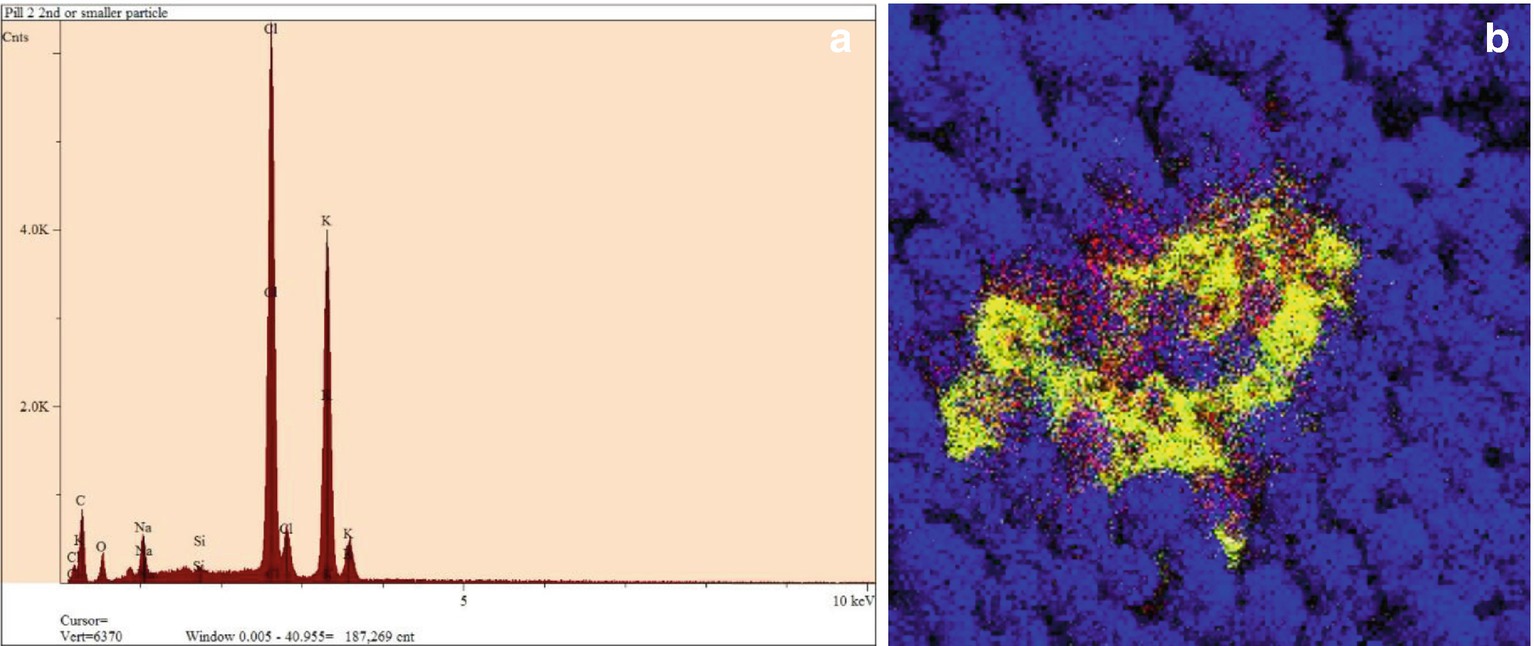
EDS spectrum and EDS mapping. (a) An EDS elemental spectrum, with the various peaks labeled for the elements they represent. (b) An x-ray dot map (or x-ray-based elemental image) of an organic powder displaying a contaminating material. Blue represents where carbon is found in the sample. Powder particles are detected in approximate shape within the blue field. The contamination is seen as yellow (represents the element sulfur) and red (represents the element chlorine). Black represents x-ray shadowing (meaning none of those x-ray are making it to the detector)
In contrast to EDS is another technique known as wavelength dispersive x-ray spectroscopy (WDS), in which x-rays are diffracted to allow analysis at a certain wavelength. WDS has traditionally been better when one analyzes for a specific element with high frequency and when one needs to know the exact concentration of that one element.
Since the SEM works in a scanning fashion, restoring its electron probe in a predictable and reproducible way, we can choose specific elements from the spectrum and record a 2-D array of element dots, from which an elemental map can be generated to show distribution of compositions (Fig. 32.5b). From EDS maps, we can know not only what elements are present but how much of that element is present and precisely where that element is in the sample.
32.2.5 Atomic Force Microscopy

Schematic of a typical AFM instrument
Although proving to have similar minimum resolution to electron microscopy, AFM finds many advantages over EM and other microscopy techniques. First, AFM measures the true height from the sample surface, which is needed to generate a 3-D surface profile. Second, AFM is not limited by the environment it operates in. Conditions such as vacuum, ambient air, different humidity, elevated or depressed temperature, and even in liquid medium all work well for AFM. Especially in liquid media, many biological macromolecules and living organism studies are possible [11]. Third, because the tip physically touches the sample, a variety of interactions and microscale forces can be measured [12].
Imagine when a tip is brought close to the surface, forces between the tip and surface constantly change as the tip gets closer (repulsive, long range electrostatic, etc.), touches the surface (capillary, van der Waals attraction, etc.), indents into the surface (various nanomechanical, etc.), and breaks away from the surface (adhesive, etc.). As the tip scans laterally, frictional forces also can be detected by quantifying the torsion of the cantilever.
AFM was first introduced to the food science field in 1993 with research work focusing on monitoring food protein changes. Since then, AFM applications have expanded to many areas of food science and technology, such as qualitative imaging of polysaccharides and proteins to understand their conformation and organization in certain environments, quantitative structure analysis on complex food systems (e.g., mechanical strength of food gels) to correlate with functionality, probing molecular interactions (e.g., interaction between protein and surfactant as co-emulsifiers), and molecular manipulations to observe the reactions among food macromolecules [13].
32.3 Chemical Imaging
32.3.1 Introduction

Schematic of chemical imaging
32.3.2 Fourier Transform Infrared Microscopy
Chemical imaging with FTIR microscopy employs IR light (mid- or near-infrared) as the incident radiation. Because of the potential absorption of IR by optical components along the beam path, no transmission type of lenses is used in FTIR microscopy (like a regular light microscope, as described in Sect. 32.2.2). Spherical or parabolic mirrors are used to focus the light, and the same optical resolution limits apply as described in Eq. 32.1. Therefore, if imaging in mid-IR (2.5–50 μm), FTIR microscopy can provide chemical maps with theoretical spatial resolution of less than 1.5 μm. However, in practical application, the resolution limit of FTIR microscopy is close to 5–10 μm when selecting functional peaks with different wavelength from the spectra.
Most FTIR microscopes adopt a point-to-point scan design, meaning the detector records only one spectrum at a time when the sample is being raster scanned. A full chemical map (e.g., 100 × 100 spectra) could take 30 min – 2 h (or longer depending on the spectral resolution and pixel settings), including the time of scanning and data recording. In 1995, the introduction of the focal plane array detector (FPA) to the FTIR microscope brought IR imaging to a whole new level [15]. A FPA detector contains a 2-D array of photo-sensitive elements (e.g., mercury cadmium telluride, MCT) with each capable of capturing a complete but totally separate IR spectrum. The detector array can be anywhere from 16 × 16 to 128 × 128 elements, enabling chemical image acquisition of up to 16,384 pixels. The Digilab Stingray FPA system had the best theoretical spatial resolution of 5.5 μm using a 36× objective. Because all spectra are collected simultaneously, the time it takes to complete a whole chemical map equals the acquisition of one single spectrum, which can be from a few seconds to a few minutes, dramatically faster than traditional IR imaging.
32.3.3 Confocal Raman Microscopy
As introduced in Chap. 8 (Sect. 8.5), Raman scattering is intrinsically weak. For Raman microscopy, because the available radiation is focused into a much smaller area, to avoid thermal damage in the sample from the laser, the effective Raman scattering is even weaker, making Raman microscopy a much less appealing technique. A great leap was seen recently in Raman microscopy technology with the development of ultrahigh throughput spectrometers and high quantum efficiency charge coupled devices (CCDs) detectors. A high-resolution Raman image (e.g., a 200 × 200 pixel scan or a 40000 spectral collection) could be acquired within a few minutes or even faster, comparing to a few hours with the old generation Raman microscope [17].
As described in Chap. 8, Raman scattering is independent of excitation wavelength, meaning visible lasers can be employed for Raman experiments, which makes the design of a Raman microscope much easier than FTIR. A regular light microscope can be readily equipped with introducing an incident laser and a mechanism to collect back scattering to enable Raman measurement.
Because visible light (much shorter wavelength than IR) can be used for Raman microscopy, image resolution can be much higher than FTIR imaging. With a green laser (e.g., 532 nm) and an oil immersion objective (e.g., NA = 1.3), the resolution limit of a Raman image can be in the 200–300 nm range.
Confocal Raman microscopy has been used extensively in food research [18–20]. However, as described in Chap. 8, fluorescence is often troublesome in image acquisition, especially in food systems with natural ingredients. Using a longer wavelength laser (e.g., 785 nm), defocusing of the incident beam, and applying pre-imaging bleaching are common ways to reduce fluorescence, but image resolution may be deteriorated.
32.3.4 Confocal Laser Scanning Microscopy
Confocal laser scanning microscopy (CLSM) is one of the four types of confocal microscopy techniques (the other three are spinning-disk, micro-lens enhanced, and programmable array microscopes), which provide high-resolution chemical images based on fluorescence emission from the sample.

Schematic of a confocal microscope
With this configuration, only light coming from the focal plane can be recorded by the detector. No background radiation from below or above the focal plane reaches the detector, which gives the recorded images a much sharper appearance. However, one limitation of the confocal setup is that the field of view is significantly smaller due to the size of the pinhole. Therefore, a scanning mechanism, typically through a set of vibrating mirrors, is often incorporated to provide images with a large field of view. The mirrors vibrate through piezoelectric elements, capable of providing scanning speed of 1800 Hz (lines/s) or faster. The entire focusing system (anything above the sample) is usually capable of moving in the vertical direction, allowing image acquisition at different focal planes. A 3-D image then can be generated by stacking images acquired from many focal planes.
The contrast of CLSM images is based on the fluorescence intensity from the laser’s illuminating point. As described in Sect. 32.2.5, there are many ways to label the target object to give fluorescence emission. Samples are often labeled with multiple fluorophores to allow co-localization studies of a complex system.
CLSM has wide applications in biological and medical science disciplines but also finds popular applications in foods (e.g., imaging fat crystal structures, dairy products, food emulsions, food gels, plant materials, etc. [21]).
32.4 X-Ray Diffraction
Molecules, atoms, or particles arrange differently in a solid material. When they pack in an ordered fashion, with symmetrical and repetitive pattern, the solid is called a crystal. Crystalline materials are rigid, have fixed melting point, can be cleaved along a definite plane, and have anisotropic physical properties such as electrical conductivity, refractive index, and thermal expansion. In contrast, amorphous materials have short range, or no order of molecular alignment. They are less rigid, usually do not have sharp melting points, and have isotropic physical properties.

Crystal unit cell and x-ray diffraction. (a) Repeating volume elements, or unit cells in a crystal, (b) Unit cell dimension parameters, (c) Parallel planes intersecting a unit cell, and reflection of x-rays off the planes


Schematic of powder diffraction. (a) Simple schematic of an x-ray diffractometer. (b) XRD spectrum of crystalline cellulose. Dotted line shows the residual amorphous phase.
X-ray diffraction patterns are characteristic of unit cell types and other structural properties of the crystals (e.g., lattice parameters, phase identity, crystallinity, composition, etc.). Figure 32.11b is a typical XRD spectrum for crystalline cellulose which is isolated from plant cell wall materials (from cotton linter in this case).
X-ray diffraction is a powerful tool for food research. Wide applications are found in carbohydrates (e.g., sugar, polysaccharides, etc.) and lipid/fats areas since these materials can easily form crystalline structures under application conditions [24, 25].
32.5 Tomography
32.5.1 Introduction
The word tomography is based on the two Greek words, tomos (meaning slice or section) and graphe (meaning to draw or write). The process of tomography, then, is the reconstructing of the original material, or specimen, from either a series of physical sections (through microtomy or sequential removal from the bulk) of that specimen or from a series of “optical” sections. Though tomography was originally done methodically by hand, the general practice now is to use computer assistance, hence, the term computer-assisted tomography. Tomography can be done using any of several possible mechanisms, such as confocal light microscopy, electron microscopy, radio frequency waves (MRI), or x-ray microscopy.
32.5.2 X-Ray Computed Tomography
X-ray computed tomography (CT) [older term is computerized axial tomography (CAT)] employs x-rays as the imaging agent to generate a 3-D digital image of the specimen. As the x-ray strikes through the object, a 2-D shadow image is collected on the detector, with contrast proportional to the x-ray attenuation or the physical density of the sample. The sample is rotated in single axis, and multiple images are collected with the orientation. A special computing algorithm (digital geometry processing) is applied to the series of 2-D images to construct a 3-D image that shows the inside of the specimen.
CT is both qualitative and quantitative. CT images can be rendered in both surface and volume modes. Segmentation can be applied to the images to render structures with similar density. The resolution of CT is mostly dependent on the x-ray beam size and the detector parameters. With a microscopic CT system, image resolution can be achieved in the range of a few micrometers.
CT is predominantly used in medical field but has found more and more applications in food research, e.g., to visualize fillings inside a chocolate cookie, to quantify air cell size and cell wall thickness of a gluten-free bread, to monitor bubble formation of an icing, and to study salt dissolution in a cookie dough.
32.6 Case Studies
32.6.1 Fat Blends
One trend in fat-/oil-related food research is to reduce the amount of saturated fat. Saturated fat forms unique crystal structures at room temperature, which not only acts as the framework of the blends to give desired physical functionality but also provides a network to hold liquid oil. Reducing or replacing the saturated fat, but keeping the same functionality, demands a thorough understanding of the fat crystal structure. Except for ingredients, processing conditions also may be adjusted to allow manipulation of fat crystal formation.

CLSM of fat crystal structures. (a) Varying cooling rate. (b) Different structuring agent. (c) Varying liquid/saturated fat ratio. (d) Same structuring agent but with varying concentration
32.6.2 Food Emulsions

Imaging characterization of emulsions with different lecithin: Top two-TEM; Bottom two-CLSM
32.7 Summary
Key characteristics of tools to examine food microstructure
|
Microstructure tool |
Imaging agent |
Typical resolution |
Key information provided |
|---|---|---|---|
|
Light microscope |
Visible light |
~200 nm |
Morphology. Composition with histology |
|
Fluorescence microscope |
Visible light |
~200 nm |
Composition |
|
SEM |
Electrons |
Sub-nm |
Surface morphology |
|
EDS |
X-rays |
Sub-nm |
Elemental composition. Elemental distribution |
|
AFM |
Sharp tip |
Sub-nm |
Surface morphology. Interfacial forces |
|
FTIR microscope |
IR light |
5–10 mm |
Chemical distribution |
|
Confocal Raman microscope |
Visible laser |
~200 nm |
Chemical distribution |
|
CLSM |
Visible laser |
~200 nm |
Chemical distribution |
|
XRD |
X-rays |
20–50 μm |
Crystallinity |
|
CT |
X-rays |
5–10 μm |
3-D morphology |
Acronyms
- 2-D
-
Two dimensional
- 3-D
-
Three dimensional
- AFM
-
Atomic force microscopy
- CAT
-
Computerized axial tomography
- CCD
-
Charge coupled device
- CLSM
-
Confocal laser scanning microscopy
- CMC
-
Critical micelle concentration
- CT
-
Computed tomography
- DIC
-
Differential interference contrast
- EDS
-
Energy dispersive spectroscopy
- EM
-
Electron microscopy
- E-SEM
-
Environmental scanning electron microscopy
- FPA
-
Focal plane array
- FTIR
-
Fourier transform infrared
- IR
-
Infrared
- LM
-
Light microscopy
- SEM
-
Scanning electron microscopy
- TEM
-
Transmission electron microscopy
- XRD
-
X-ray diffraction
32.8 Study Questions
- 1.
What is the definition of “resolution” with regard to microscopy? How is the resolution of an optical microscope determined?
- 2.
What is the main reason that electron microscopes can work at much higher magnifications (or resolution) than light microscopes?
- 3.
Why do we apply a conductive coating to samples examined by an SEM? Why is a conductive coating usually not needed when examining samples using either a low vacuum SEM or an environmental SEM?
- 4.
When using energy-dispersive x-ray spectroscopy (EDS), what carry the information telling us the elemental content of the sample, and where do they come from?
- 5.
FT-Raman is often an option when sample has strong fluorescence. Why is it not used in Raman microscope?
- 6.
What is “tomography” and what advantages does it have over other imaging techniques? How does computer-assisted x-ray tomography create a 3-D image?
- 7.
You are working on a project to reduce the sugar content in gummy candies. You replaced some sugar with high-intensity sweetener and added some starch to try to maintain the elastic property. However, the candy does not look and taste like the normal gummy candy. You are asked to understand the candy’s microstructure. What would be your experimental plan to do the characterization?

Open Access This chapter is licensed under the terms of the Creative Commons Attribution-NonCommercial 2.5 International License (http://creativecommons.org/licenses/by-nc/2.5/), which permits any noncommercial use, sharing, adaptation, distribution and reproduction in any medium or format, as long as you give appropriate credit to the original author(s) and the source, provide a link to the Creative Commons license and indicate if changes were made.
The images or other third party material in this chapter are included in the chapter's Creative Commons license, unless indicated otherwise in a credit line to the material. If material is not included in the chapter's Creative Commons license and your intended use is not permitted by statutory regulation or exceeds the permitted use, you will need to obtain permission directly from the copyright holder.