In the previous chapter we explained by what
means the cosmological parameters may be determined, and what
progress has been achieved in recent years. This might have given
the impression that, with the determination of the values for
Ω m,
Ω Λ etc., cosmology is nearing its
conclusion. As a matter of fact, for several decades cosmologists
have considered the determination of the density parameter and the
expansion rate of the Universe as their prime task, and now this
goal has largely been achieved. However, from this point on, the
future evolution of the field of cosmology will probably proceed in
two directions. First, we will try to uncover the nature of dark
energy and to gain new insights into fundamental physics along the
way. Second, astrophysical cosmology is much more than the mere
determination of a few parameters. We want to understand how the
Universe evolved from a very primitive initial state, as seen in
the almost isotropic CMB radiation, into what we are observing
around us today—galaxies of different morphologies, luminosities
and spectral properties, the large-scale structure of their
distribution, groups and clusters of galaxies, active galaxies, and
the intergalactic medium. We seek to study the formation of stars
and of metals, the cosmic history of star formation, and also the
processes that reionized and enriched the intergalactic medium with
heavy elements.
The boundary conditions for studying these
processes are now very well defined. Until about the year 2000, the
cosmological parameters in models of galaxy evolution, for
instance, could be chosen from within a large range, because they
had not been determined sufficiently well at that time. That
allowed these models more freedom to adjust the model outcomes such
that they best fit with observations. Today however, a successful
model needs to make predictions compatible with observations, but
using the parameters of the standard model. In terms of the
cosmological parameters, there is little freedom left in designing
such models. In other words, the stage on which the formation and
evolution of objects and structure takes place is prepared, and now
the cosmic play can begin.
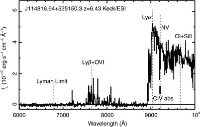
Fig. 9.1
Spectrum of a QSO at the high redshift of
z = 6. 419. Like many other
QSOs at very high redshift, this source was discovered with the
Sloan Digital Sky Survey. The spectrum was obtained with the Keck
telescope. The redshifted Lyα line is clearly visible, its blue
side ‘eaten’ away by intergalactic absorption. Almost all radiation
bluewards of the central wavelength of the Lyα line is absorbed; however, a low
level of this radiation is getting through, as is most clearly seen
from the Lyβ line. For
λ ≤ 7200 Å the spectral
flux is consistent with zero; intergalactic absorption is too
strong here. Source: X. Fan et al. 2003, A Survey of z > 5.7 Quasars in the Sloan
Digital Sky Survey. II. Discovery of Three Additional Quasars at z
> 6, AJ 125, 1649, p. 16554, Fig. 6. ©AAS. Reproduced
with permission
Progress in recent years, with developments in
instrumentation having played a vital role, has allowed us to
examine the Universe at very high redshift. An obvious indication
of this progress is the increasingly high maximum redshift of
sources that can be observed; as an example, Fig. 9.1 presents the spectrum
of a QSO at redshift z = 6. 419 whose precise redshift was
measured from molecular CO lines. Today, we know quite a few
galaxies at redshift z > 6, i.e., we observe these
objects at a time when the Universe had less than 10 % of its
current age and when the density of the neutral hydrogen in the
intergalactic medium was apparently considerably higher than at
later epochs, as concluded from the very strong absorption blueward
of the Lyα emission line
(see Fig. 9.1). As we shall see, the detection of galaxies
at even higher redshifts has been claimed. Besides larger
telescopes, which enabled these deep images of the Universe,
gaining access to new wavelength domains is of particular
importance for our studies of the distant Universe. This can be
seen, for example, from the fact that the optical radiation of a
source at redshift z ∼ 1 is
shifted into the NIR. Because of this, near-infrared astronomy is
about as important for galaxies at z ≳ 1 as optical astronomy is for the
local Universe. Furthermore, the development of sub-millimeter
astronomy has provided us with a view of sources that are nearly
completely hidden to the optical eye because of strong dust
absorption.
In this chapter, we will attempt to provide an
impression of astronomy of the distant Universe, and shed light on
some interesting aspects that are of particular importance for our
understanding of the evolution of the Universe, whereas in
Chap. 10, we will try to provide an
impression of our theoretical understanding of the evolution of
galaxies throughout the Universe. Both, observational as well as
theoretical and numerical studies, are currently very rapidly
developing fields of research, so we will simply address some of
the main topics in this field today. We begin in Sect. 9.1 with a discussion of
methods to specifically search for high-redshift galaxies, and we
will then focus on a method by which galaxy redshifts can be
determined solely from photometric information in several bands
(thus, from the color of these objects). This method can be applied
to deep multi-band sky images, and we will present some of the
results from deep HST surveys, described in Sect. 9.2. We will also
emphasize the importance of gravitational lenses as ‘natural
telescopes’, which provide us with a deeper view into the Universe
due to their magnification effect.
Gaining access to new wavelength domains paves
the way for the discovery of new kinds of sources; in
Sect. 9.3 we
will present high-redshift galaxy populations, some of which have
been identified by sub-millimeter and NIR observations. Some key
properties of the high-redshift galaxy population will be described
in Sect. 9.4,
including their luminosity function; as will be shown there, the
properties of galaxies in the early phases of our Universe are
quite different from the present galaxies. In Sect. 9.5 we will show that,
besides the CMB, background radiation also exists at other
wavelengths, but whose nature is considerably different from that
of the CMB; recent progress has allowed us to identify the nature
of these cosmic backgrounds. Then, in Sect. 9.6, we will focus on the
history of cosmic star formation, and show that at redshift
z ≳ 1 the Universe was much
more active than it is today—in fact, most of the stars that are
observed in the Universe today were already formed in the first
half of cosmic history. This empirical discovery is one of the
aspects that one attempts to explain in the framework of models of
galaxy formation and evolution. Finally, in Sect. 9.7 we will discuss the
sources of gamma-ray bursts. These are explosive events which, for
a very short time, appear brighter than all other sources of gamma
rays on the sky put together. For about 25 years the nature of
these sources was totally unknown; even their distance estimates
were spread over at least seven orders of magnitude. Only since
1997 has it been known that these sources are of extragalactic
origin.
9.1 Galaxies at high redshift
In this section we will first consider how
distant galaxies can be found, and how to identify them as such.
The properties of these high-redshift galaxies can then be compared
with those of galaxies in the local Universe, which were described
in Chap. 3. The question then arises as to
whether galaxies at high z,
and thus in the early Universe, look like local galaxies, or
whether their properties are completely different. One might, for
instance, expect that the mass and luminosity of galaxies are
evolving with redshift since, as we have seen in Sect. 7.5.2, the mass function of dark
matter halos changes during cosmic evolution. Examining the galaxy
population as a function of redshift, one can trace the history of
global cosmic star formation and analyze when most of the stars
visible today have formed, and how the density of galaxies changes
as a function of redshift. We will investigate some of these
questions in this and the following sections.
How to find
high-redshift galaxies? Until about 1995 only a few galaxies
with z > 1 had been
known; most of them were radio galaxies discovered by optical
identification of radio sources. The most distant normal galaxy
with z > 2 then was the
source of the giant luminous arc in the galaxy cluster Cl 2244−02
(see Fig. 6.49). Very distant galaxies are
expected to be faint, and so the question arises of how galaxies at
high z can be detected at
all.
The most obvious answer to this question may
perhaps be by spectroscopy of a sample of faint galaxies. This
method is not feasible though, since galaxies with R ≲ 22 have redshifts z ≲ 0. 5, and spectra of galaxies with
R > 22 are observable
only with 4-m telescopes and with a very large investment of
observing time.1
Also, the problem of finding a needle in a haystack arises: most
galaxies with R ≲ 24. 5
have redshifts z ≲ 2 (a
fact that was not established before 1995), so how can we detect
the small fraction of galaxies with larger redshifts?
Narrow-band
photometry. A more systematic method that has been applied
is narrow-band photometry. Since hydrogen is the most abundant
element in the Universe, one expects that some fraction of galaxies
feature a Lyα emission line
(as do all QSOs). By comparing two sky images, one taken with a
narrow-band filter centered on a wavelength λ, the other with a broader filter also
centered roughly on λ, this
line emission can be searched for specifically. If a galaxy at
 has
a strong Lyα emission line,
it should be particularly bright in the narrow-band image in
comparison to the broad-band image, relative to other sources. This
search for Lyα emission
line galaxies had been almost without success until the mid-1990s.
Among other reasons, one did not know what to expect, e.g., how
faint galaxies at z ≳ 3 are
and how strong their Lyα
line would be. Another reason, which was found only later, was the
leakage of the narrow-band filters for radiation at shorter and
longer wavelength—the transmission of these filters was not close
enough to zero for wavelengths outside the considered narrow range.
We will see later that more recent narrow-band photometric surveys
have indeed uncovered a population of high-redshift galaxies.
has
a strong Lyα emission line,
it should be particularly bright in the narrow-band image in
comparison to the broad-band image, relative to other sources. This
search for Lyα emission
line galaxies had been almost without success until the mid-1990s.
Among other reasons, one did not know what to expect, e.g., how
faint galaxies at z ≳ 3 are
and how strong their Lyα
line would be. Another reason, which was found only later, was the
leakage of the narrow-band filters for radiation at shorter and
longer wavelength—the transmission of these filters was not close
enough to zero for wavelengths outside the considered narrow range.
We will see later that more recent narrow-band photometric surveys
have indeed uncovered a population of high-redshift galaxies.9.1.1 Lyman-break galaxies (LBGs)
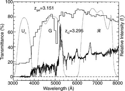
Fig. 9.2
Principle of the Lyman-break method. The
histogram shows the synthetic spectrum of a galaxy at z = 3. 15, generated by models of
population synthesis; the spectrum belongs to a QSO at slightly
higher redshift. Clearly, the decline of the spectrum at
λ ≤ 912(1 + z)Å is noticeable. Furthermore, we see
that the flux for λ ≤ 1216(1 + z)Å is reduced relative to the
radiation on the red side of the Lyman-α emission line due to the integrated
absorption of the intergalactic Lyman-α forest. For higher redshift sources,
this latter effect becomes stronger, so that for them the break
occurs already at a rest wavelength of λ = 1216 Å. The three dotted curves are the transmission
curves of three broad-band filters, chosen such that one of them
(Un) blocks all photons with wavelengths above the
Lyman-break. The color of this galaxy would then be blue in
 , and very red in
Un − G. Source: C.C. Steidel et al. 1995,
Lyman Imaging of High-Redshift
Galaxies. III. New Observations of Four QSO Fields, AJ 110,
2519, p. 2520, Fig. 1. ©AAS. Reproduced with permission
, and very red in
Un − G. Source: C.C. Steidel et al. 1995,
Lyman Imaging of High-Redshift
Galaxies. III. New Observations of Four QSO Fields, AJ 110,
2519, p. 2520, Fig. 1. ©AAS. Reproduced with permission
, and very red in
Un − G. Source: C.C. Steidel et al. 1995,
Lyman Imaging of High-Redshift
Galaxies. III. New Observations of Four QSO Fields, AJ 110,
2519, p. 2520, Fig. 1. ©AAS. Reproduced with permission
Fig. 9.3
Top
panel: A U-band drop-out galaxy. It is clearly detected in
the two redder filters, but vanishes almost completely in the
U-filter. Bottom panel: In
a single CCD frame, a large number of candidate Lyman-break
galaxies ( ∼ 150) are found. They are marked with circles here; their density is about 1
per square arcminute. Credit: C.C. Steidel
The method.
The breakthrough was obtained with a method that became known as
the Lyman-break method.
Since hydrogen is so abundant and its ionization cross section so
large, one can expect that photons with λ < 912 Å are very heavily absorbed
by neutral hydrogen in its ground state. Therefore, photons with
λ < 912 Å have a low
probability of escaping from a galaxy without being absorbed.
Intergalactic absorption also contributes. In
Sect. 5.7 we saw that each QSO spectrum
features a Lyα forest and
often also Lyman-limit absorption. The intergalactic gas absorbs a
large fraction of photons emitted by a high-redshift source at
λ < 1216 Å, and
virtually all photons with a rest-frame wavelength λ ≲ 912 Å. As also discussed in
Sect. 8.5.2, the strength of this
absorption increases with increasing redshift. Combining these
facts, we conclude that spectra of high-redshift galaxies should
display a distinct feature—a ‘break’—at λ = 912 Å for redshifts z ≲ 4, and for higher redshifts, the
break shifts more towards λ = 1216 Å. Furthermore, radiation with
λ ≲ 912 Å should be
strongly suppressed by intergalactic absorption, as well as by
absorption in the interstellar medium of the galaxies themselves,
so that only a very small fraction of these ionizing photons will
reach us.
From this, a strategy for the detection of
galaxies at z ≳ 3 emerges.
We consider three broad-band filters with central wavelengths
λ
1 < λ
2 < λ
3, where their spectral ranges are chosen to not (or
only marginally) overlap. If λ 1 ≲ (1 + z)912 Å ≲ λ 2, a galaxy containing
young stars should appear relatively blue as measured with the
filters λ 2 and
λ 3, and be
virtually invisible in the λ 1-filter: because of the
absorption, it will drop out of the λ 1-filter (see
Fig. 9.2). For
this reason, galaxies that have been detected in this way are
called Lyman-break galaxies
(LBGs) or drop-outs.
An example of this is displayed in Fig. 9.3.
Large samples of
LBGs. The method was first applied systematically in 1996,
using the filters specified in Fig. 9.2. As can be read from
Fig. 9.4, the
expected location of a galaxy at z ∼ 3 in a color-color diagram with
this set of filters is nearly independent of the type and star
formation history of the galaxy. Hence, sources in the relevant
region of the color-color diagram are very good candidates for
being galaxies at z ∼ 3.
The redshift needs to be verified spectroscopically, but the
crucial point is that the color selection of candidates yields a
very high success rate per observed spectrum, and thus
spectroscopic observing time at the telescope is spent very
efficiently in confirming the redshift of distant galaxies. With
the commissioning of the Keck telescope (and later also of other
telescopes of the 10-m class), spectroscopy of galaxies with
B ≲ 25 became possible (see
Fig. 9.5).
Employing this method, thousands of galaxies with
2. 5 ≲ z ≲ 3. 5 have been
detected and spectroscopically verified to date.

Fig. 9.4
Left
panel: Evolutionary tracks of galaxies in the ( ) – (Un − G)
color-color diagram, for different types of galaxies, as obtained
from population synthesis models. All evolutionary tracks start at
z = 0, and the symbols along the curves mark intervals
of Δ z = 0. 1. The colors
of the various galaxy types are very different at lower redshift,
but for z ≥ 2. 7, the
evolutionary tracks for the different types nearly coincide—a
consequence of the Lyα
absorption in the intergalactic medium. Hence, a color selection of
galaxies in the region between the dotted and dashed curves should select galaxies
with z ≥ 3. Indeed, this
selection of candidates has proven to be very successful; thousands
of galaxies with z ∼ 3 have
been spectroscopically verified. Right panel: The same color-color
diagram, with objects selected from one survey field. The
green and yellow shaded regions show the
selection criteria for z ∼ 3 Lyman-break galaxies, the
cyan and magenta regions indicate the selection
windows for galaxies with z ∼ 2. 2 and z ∼ 1. 7, respectively. The symbols are
coded according to the brightness of the sources, and triangles denote sources for which only
lower limits in the Un − G color were obtained. Source:
Left: C.C. Steidel et
al. 1995, Lyman Imaging of
High-Redshift Galaxies. III. New Observations of Four QSO
Fields, AJ 110, 2519, p. 2522, Fig. 2. ©AAS. Reproduced with
permission. Right:
C.C. Steidel et al. 2004, A Survey of Star-forming Galaxies in
the 1. 4 ≲ z ≲ 2. 5
Redshift Desert: Overview,
ApJ 604, 534, p. 537, Fig. 1. ©AAS. Reproduced with
permission
) – (Un − G)
color-color diagram, for different types of galaxies, as obtained
from population synthesis models. All evolutionary tracks start at
z = 0, and the symbols along the curves mark intervals
of Δ z = 0. 1. The colors
of the various galaxy types are very different at lower redshift,
but for z ≥ 2. 7, the
evolutionary tracks for the different types nearly coincide—a
consequence of the Lyα
absorption in the intergalactic medium. Hence, a color selection of
galaxies in the region between the dotted and dashed curves should select galaxies
with z ≥ 3. Indeed, this
selection of candidates has proven to be very successful; thousands
of galaxies with z ∼ 3 have
been spectroscopically verified. Right panel: The same color-color
diagram, with objects selected from one survey field. The
green and yellow shaded regions show the
selection criteria for z ∼ 3 Lyman-break galaxies, the
cyan and magenta regions indicate the selection
windows for galaxies with z ∼ 2. 2 and z ∼ 1. 7, respectively. The symbols are
coded according to the brightness of the sources, and triangles denote sources for which only
lower limits in the Un − G color were obtained. Source:
Left: C.C. Steidel et
al. 1995, Lyman Imaging of
High-Redshift Galaxies. III. New Observations of Four QSO
Fields, AJ 110, 2519, p. 2522, Fig. 2. ©AAS. Reproduced with
permission. Right:
C.C. Steidel et al. 2004, A Survey of Star-forming Galaxies in
the 1. 4 ≲ z ≲ 2. 5
Redshift Desert: Overview,
ApJ 604, 534, p. 537, Fig. 1. ©AAS. Reproduced with
permissionFrom the spectra shown in Fig. 9.5, it also becomes
apparent that not all galaxies that fulfill the selection criteria
also show a Lyα emission
line, which provides one of the explanations for the lack of
success in earlier searches for high-redshift galaxies using
narrow-band filters. The spectra of the high-redshift galaxies
which were found by this method are very similar to those of
starburst galaxies at low redshift. It should come as no surprise
that the galaxies selected by the drop-out technique feature active
star formation, since it was required that the spectrum on the red
side of the break—i.e., at (rest-frame) wavelengths above
1216 Å—shows a blue spectrum. Such a blue spectrum in the
rest-frame UV is produced only by a stellar population which
features active star formation. Furthermore, the luminosity of
galaxies in the rest-frame UV and blue range strongly depends on
the star-formation rate, so that preferentially galaxies with the
highest (unobscured—see below) star-formation rate are
selected.
This is a prominent example of the effect that
the physical properties of objects selected depend on the selection
criteria. One must always bear in mind that, when comparing galaxy
populations detected by different methods, the properties can
differ substantially. One of the challenges of studies of
(high-redshift) galaxies is to get a coherent picture of the galaxy
population from samples with a vast variety of selection
methods.
The correlation
function and halo masses of LBGs. For a large variety of
objects, and over a broad range of separations, the spatial
correlation function of objects can be described by the power
law (7.28), with a slope of typically
γ ∼ 1. 7. However, the
amplitude of this correlation function varies between different
classes of objects. For example, we saw in Sect. 8.2.4 that the amplitude of the
power spectrum of galaxy clusters is larger by about a factor 7
than that of galaxies (see Fig. 8.23); the same ratio holds of
course for the corresponding correlation functions. As we argued
there, the strength of the correlation depends on the mass of
objects; in the simple picture of biasing shown in
Fig. 7.22, the correlation of objects is
larger the rarer they are. High-mass peaks exceeding the density
threshold needed for gravitational collapse have a lower mean
number density than low-mass peaks, so they are therefore expected
to be more biased (see Sect. 8.1.3) and thus more strongly
correlated.
If we now assume that each galaxy lives in a dark
matter halo, we can estimate the dark halo mass from the observed
correlation function of these galaxies. As we discussed in
Sect. 7.6.3, dark matter halos have
clustering properties which differ from the clustering of the
underlying matter density field, and we described that in terms of
the halo biasing b
h(M, z),
which is a function of halo mass and redshift. The dark matter
correlation function can be determined quite accurately from
numerical simulations. The ratio of the observed correlation
function to the dark matter correlation function then yields the
square of the halo bias parameter (7.68), and comparing that to the
numerically-determined function b h(M, z), the corresponding halo mass can be
obtained.

Fig. 9.5
Spectra of two galaxies at z ∼ 3, detected by means of the
U-drop-out technique. Below each spectrum, the spectrum of a nearby
starburst galaxy (NGC 4214)—shifted to the corresponding
redshift—is plotted; it becomes apparent that the spectra of
galaxies at z ∼ 3 are very
similar to those of present-day star-forming galaxies. One of the
two U-drop-out galaxies features a strong Lyα emission line, the other shows
absorption at the respective wavelength. Source: C.C. Steidel
et al. 1996, Spectroscopic
Confirmation of a Population of Normal Star-forming Galaxies at
Redshifts z > 3, ApJ 462, L17, PLATE L3, Fig. 1. ©AAS.
Reproduced with permission
Considering the spatial distribution of LBGs, we
find a large correlation amplitude. The (comoving) correlation
length of LBGs at redshifts 1. 5 ≲ z ≲ 3. 5 is r 0 ∼ 4. 2h −1 Mpc, i.e., not very
different from the correlation length of L ∗-galaxies in the present
Universe. Since the bias factor of present-day galaxies is about
unity, implying that they are clustered in a similar way as the
dark matter distribution, this result then implies that the bias of
LBGs at high redshift must be considerably larger than unity. This
conclusion is based on the fact that the dark matter correlation at
high redshifts (on large scales, i.e., in the linear regime) was
smaller than today by the factor D +
2(z), where
D + is the
growth factor of linear perturbations introduced in
Sect. 7.2.2. Thus we conclude that LBGs
are rare objects and thus correspond to high-mass dark matter
halos. Comparing the observed correlation length r 0 with numerical
simulations, the characteristic halo mass of LBGs can be
determined, yielding ∼ 3 × 10¹¹ M ⊙ at redshifts
z ∼ 3,
and ∼ 1012 M
⊙ at z ∼ 2.
Furthermore, the correlation length is observed to increase with
the luminosity of the LBG, indicating that more luminous galaxies
are hosted by more massive halos, which are more strongly biased
than less massive ones. If these results are combined with the
observed correlation functions of galaxies in the local Universe
and at z ∼ 1, and with the
help of numerical simulations, then this indicates that a typical
high-redshift LBG will evolve into a massive elliptical galaxy by
today.
Proto-clusters. Furthermore, the
clustering of LBGs shows that the large-scale galaxy distribution
was already in place at high redshifts. In some fields the observed
overdensity in angular position and galaxy redshift is so large
that one presumably observes galaxies which will later assemble
into a galaxy cluster—hence, we observe some kind of proto-cluster.
We have already shown such a proto-cluster in Fig. 6.71. Galaxies in such a
proto-cluster environment seem to have about twice the stellar mass
of those LBGs outside such structures, and the age of their stellar
population appears older by a factor of two. This result indicates
that the stellar evolution of galaxies in dense environments
proceeds faster than in low-density regions, in accordance with
expectations from structure formation. It also reveals a dependence
of galaxy properties on the environment, which we have seen before
manifested in the morphology-density relation (see
Sect. 6.7.2). Proto-clusters of galaxies
have also been detected at higher redshifts up to z ∼ 6, using narrow-band imaging
searches for Lyman-alpha emission galaxies (see below).
Satellite galaxies
at high redshifts. Whereas the clustering of LBGs is well
described by the power law (7.28) over a large range of scales,
the correlation function exhibits a significant deviation from this
power law at very small scales: the angular correlation function
exceeds the extrapolation of the power law from larger angles at
Δ θ ≲ 7″, corresponding to
comoving length-scales of ∼ 200 kpc. It thus seems that this scale
marks a transition in the distribution of galaxies. To get an idea
of the physical nature of this transition, we note that this
length-scale is about the virial radius of a dark matter halo with
M ∼ 3 × 10¹¹
M ⊙, i.e., the
mass of halos which host the LBGs. On scales below this virial
radius, the correlation function thus no longer describes the
correlation between two distinct dark matter halos. An
interpretation of this fact is provided in terms of merging: when
two galaxies and their dark matter halos merge, the resulting dark
matter halo hosts both galaxies, with the more massive one close to
the center and the other one as ‘satellite galaxy’. The correlation
function on scales below the virial radius thus indicates the
clustering of galaxies within the same halo, whereas on larger
scales, where it follows the power-law behavior, it indicates the
correlation between different halos. Note that this effect is also
well described in the halo model which we discussed in
Sect. 7.7.3. On large scales, the
correlation function is dominated by the two-halo term, whereas on
smaller scales, the one-halo term takes over. The transition
between these two regimes, which at low redshifts occurs on scales
of several hundred kiloparsecs (see Fig. 7.27), is at smaller scales for
high-redshift galaxies, since the high-mass population of galaxy
clusters has not formed yet at these early epochs.
Winds of
star-forming galaxies. The inferred high star-formation
rates of LBGs implies an accordingly high rate of supernova
explosions. These release part of their energy in the form of
kinetic energy to the interstellar medium in these galaxies. This
process will have two consequences. First, the ISM in these
galaxies will be heated locally, which slows down (or prevents)
further star formation in these regions. This thus provides a
feedback effect for star formation which prevents all the gas in a
galaxy from turning into stars on a very short time-scale, and is
essential for understanding the formation and evolution of
galaxies, as we shall see in Sect. 10.4.4. Second, if the amount of
energy transferred from the SNe to the ISM is large enough, a
galactic wind may be launched which drives part of the ISM out of
the galaxy into its halo. Evidence for such galactic winds has been
found in nearby galaxies, for example from neutral hydrogen
observations of edge-on spirals which show an extended gas
distribution outside the disk. Furthermore, the X-ray corona of
spirals (see Fig. 3.26) is most likely linked to a
galactic wind in these systems.
Indeed, there is now clear evidence for the
presence of massive winds from LBGs. The spectra of LBGs often show
strong absorption lines, e.g., of Civ, which are blueshifted relative
to the velocity of the emission lines in the galaxy. An example of
this effect can be seen in the spectra of Fig. 9.5, where in the upper
panel the emission line of Civ is accompanied by an absorption
to the short-wavelength side of the emission line. Such absorption
can be produced by a wind moving out from the star-forming regions
of the galaxy, so that its redshift is smaller than that of the
emission regions. Characteristic velocities are ∼ 200 km∕s. In one
case where the spectral investigation has been performed in most
detail (the LBG cB58; see Fig. 9.17), the outflow velocity is ∼ 255 km∕s, and
the outflowing mass rate exceeds the star-formation rate. Whereas
these observations clearly show the presence of outflowing gas, it
remains undetermined whether this is a fairly local phenomenon,
restricted to the star-formation sites, or whether it affects the
ISM of the whole galaxy.
Connection to QSO
absorption lines. A slightly more indirect argument for the
presence of strong winds from LBGs comes from correlating the
absorption lines in background QSO spectra with the position of
LBGs. These studies have shown that whenever the sight-line of a
QSO passes within ∼ 40 kpc of an LBG, very strong Civ absorption lines (with column
density exceeding 1014 cm−2) are produced,
and that the corresponding absorbing material spans a velocity
range of Δ v ≳ 250 km∕s;
for about half of the cases with impact parameters within 80 kpc,
strong Civ absorption is
produced. This frequency of occurrence implies that about 1/3 of
all Civ metal absorption
lines with N ≳ 1014 cm−2 in
QSO spectra are due to gas within ∼ 80 kpc from those LBGs which
are bright enough to be included in current surveys. It is
plausible that many of the remaining 2/3 are due to fainter
LBGs.
The association of Civ absorption line systems with LBGs
by itself does not prove the existence of winds in such galaxies;
in fact, the absorbing material may be gas orbiting in the halo in
which the corresponding LBG is embedded. In this case, no outflow
phenomenon would be implied. However, in that case one might wonder
where the large amount of metals implied by the QSO absorption
lines is coming from. They could have been produced by an earlier
epoch of star formation, but in that case the enriched material
must have been expelled from its production site in order to be
located in the outer part of z ∼ 3 halos. It appears more likely
that the production of metals in QSO absorption systems is directly
related to the ongoing star formation in the LBGs. We shall see in
Sect. 9.3.5
that clear evidence for superwinds has been discovered in one
massive star-forming galaxy at z ∼ 3.

Fig. 9.6
A galaxy at z = 5. 74, which is visible in the
narrow-band filter (upper left
panel) and in the I- and z-band (located between the two
horizontal dashes), but which does not show any flux in the three
filters at shorter wavelength (lower panels). Source: Hu et
al. 1999, An Extremely
Luminous Galaxy at z = 5. 74, ApJ 522, L9, p. L10, Fig. 1.
©AAS. Reproduced with permission
Finally, we mention another piece of evidence for
the presence of superwinds in star-forming galaxies. There are
indications that the density of absorption lines in the
Lyα forest is reduced when
the sight-line to the QSO passes near a foreground LBG. This may
well be explained by a wind driven out from the LBG, pushing
neutral gas away and thus leaving a gap in the Lyα forest. The characteristic size of
the corresponding ‘bubbles’ is estimated to be ∼ 0. 5 Mpc for
luminous LBGs.
Lyman-break
galaxies at low redshifts. One might ask whether galaxies
similar to the LBGs at z ∼ 3 exist in the current Universe.
Until recently this question was difficult to investigate, since it
requires imaging of lower redshift galaxies at ultraviolet
wavelengths. With the launch of GALEX an appropriate observatory
became available with which to observe galaxies with restframe UV
luminosities similar to those of LBGs. UV-selected galaxies show a
strong inverse correlation between the stellar mass and the surface
brightness in the UV. Lower-mass galaxies are more compact than
those of higher stellar mass. On the basis of this correlation we
can consider the population of large and compact UV-selected
galaxies separately. The larger ones show a star-formation rate of
a few M ⊙∕yr; at
this rate, their stellar mass content can be built up on a
time-scale comparable to the Hubble time, i.e., the age of the
Universe. These galaxies are typically late-type spiral galaxies,
and they show a metallicity similar to our Galaxy.
In contrast, the compact galaxies have a lower
stellar mass and about the same star-formation rate, which allows
them to generate their stellar population much faster, in about
1 Gyr. Compared to normal low-redshift galaxies, their metallicity
is smaller by about a factor of 2 for a given stellar mass. In
addition, they show similar extinction and outflow properties as
the LBG at z ∼ 3. Hence,
the properties of the compact UV-selected galaxies, which are
sometimes called Lyman-break analogs , are quite similar to those
of the LBGs seen at higher redshifts, and they may indeed be
closely related to the LBG population.
Lyman-break
galaxies at high redshift. By variation of the filter set,
drop-outs can also be discovered at larger wavelengths, thus at
accordingly higher redshifts. The object selection at higher
z implies an increasingly
dominant role of the Lyα
forest whose density is a strongly increasing function of redshift
(see Sect. 8.5.2). This method has been
routinely applied with ground-based observations up to z ∼ 4. 5, yielding so-called
B-drop-outs. Galaxies at considerably higher redshifts are
difficult to access from the ground with this method. One reason
for this is that galaxies become increasingly faint with redshift,
rendering observations substantially more difficult. Furthermore,
one needs to use increasingly redder filter sets. At such large
wavelengths the night sky gets significantly brighter, which
further hampers the detection of very faint objects. For detecting
a galaxy at redshift, say, z = 5. 5 with this method, the
Lyα line, now at
λ ≈ 7900 Å, is located
right in the I-band, so that for an efficient application of the
drop-out technique only the I- and z-band filters or NIR-filters
are viable, and with those filters the brightness of the night sky
is very problematic (see Fig. 9.6 for an example of a drop-out galaxy at very
high redshift). Furthermore, candidate very high-redshift galaxies
detected as drop-outs are very difficult to verify
spectroscopically due to their very faint flux and the fact that
most of the diagnostic spectral features are shifted to the
near-IR. In spite of this, we will see later that the drop-out
method has achieved spectacular results even at redshifts
considerably higher than z ∼ 4, where the HST played a central
role.
9.1.2 Photometric redshift
Spectral
breaks. The Lyman-break technique is a special case of a
method for estimating the redshift of galaxies (and QSOs) by
multi-color photometry. This technique can be employed due to the
spectral breaks at λ = 912 Å and λ = 1216 Å, respectively. Spectra of
galaxies also show other characteristic features. As was discussed
in detail in Sect. 3.5, the broad-band energy
distribution is basically a superposition of stellar radiation (if
we ignore for a moment the presence of dust, which can yield a
substantial infrared emission from galaxies). A stellar population
of age ≳ 108 yr features a 4000 Å-break because, due to
a sudden change in the opacity at this wavelength, the spectra of
most stars show such a break at about 4000 Å (see Fig. 3.33). Hence, the radiation from a
stellar population at λ < 4000 Å is less intense than at
λ > 4000 Å; this is the
case particularly for early-type galaxies, as can be seen in
Fig. 3.36, due to their old stellar
population.
Principle of the
method. If we assume that the star-formation histories of
galaxies are not too diversified, the spectral energy distributions
of these galaxies are expected to follow certain patterns. For
example, if all galaxies had a single episode of star formation,
starting at redshift z
f and lasting for a time τ, then the spectra of these galaxies,
for a given initial mass function, would be characterized by these
two parameters, as well as the total stellar mass formed (see
Sect. 3.5); this latter quantity then
yields the amplitude of the spectrum, but does not affect the
spectral shape. When measuring the magnitude of these galaxies in
n broad-band filters, we
can form n − 1 independent
colors. Next suppose we form a multi-dimensional color-color
diagram, in which every galaxy is represented by a point in this
(n − 1)-dimensional color
space. Considering only galaxies at the present epoch, all these
points will lie on a two-dimensional surface in this
multi-dimensional space, instead of being more or less randomly
distributed.
Next, instead of plotting z = 0 galaxies, we consider the
distribution of galaxies at some higher redshift z < z f. This distribution of
points will be different, mainly due to two different effects.
First, a given photometric filter corresponds to a different
rest-frame spectral range of the galaxy, due to redshift. Second,
the ages of the stellar populations are younger at an earlier
cosmic epoch, and thus the spectral energy distributions are
different. Both of these effects will cause these redshift
z galaxies to occupy a
different two-dimensional surface in multi-color space.
Generalizing this argument further, we see that in this idealized
consideration, galaxies will occupy a three-dimensional subspace in
(n − 1)-dimensional color
space, parametrized by formation redshift z f, time-scale τ and the galaxy’s redshift
z. Hence, from the
measurement of the broad-band energy distribution of a galaxy, we
might expect to be able to determine, or at least estimate, its
redshift, as well as other properties such as the age of its
stellar population; this is the principle of the method of
photometric
redshifts.
Of course, the situation is considerably more
complicated in reality. Galaxies most likely have a more
complicated star-formation history than assumed here, and hence
they will not be confined to a two-dimensional surface at fixed
redshift, but instead will be spread around this surface. The
spectrum of a stellar population also depends on its metallicity,
as well as absorption, either by gas and dust in the interstellar
medium or hydrogen in intergalactic space (of which the Lyman-break
method makes proper use). On the other hand, we have seen in
Sect. 3.6 that the colors of current-day
galaxies are remarkably similar, best indicated by the red
sequence. Therefore, the method of photometric redshifts may be
expected to work, even if more complications are accounted for than
in the idealized example considered above.
The method is strongly aided if the galaxies have
characteristic spectral features, which shift in wavelength as the
redshift is changed. If, for example, the spectrum of a galaxy was
a power law in wavelength, then the redshifted spectrum would as
well be a power law, with the same spectral slope—if we ignore the
different age of the stellar population. Therefore, for such a
spectral energy distribution is would be impossible to estimate a
redshift. However, if the spectrum shows a clear spectral break,
then the location of this break in wavelength depends directly on
the redshift, thus yielding a particularly clean diagnostic. In
this context the 4000 Å-break and the Lyα-break play a central role, as is
illustrated in Fig. 9.7.
Calibration. In order to apply this
method, one needs to find the characteristic domains in color space
where (most of) the galaxies are situated. This can be done either
empirically, using observed energy distributions of galaxies, or by
employing population synthesis model. More precisely, a number of
standard spectra of galaxies (so-called templates) are used, which
are either selected from observed galaxies or computed by
population synthesis models. Each of these template spectra can
then be redshifted in wavelength. For each template spectrum and
any redshift, the expected galaxy colors are determined by
integrating the spectral energy distribution, multiplied by the
transmission functions of the applied filters, over wavelength [see
(A.25)]. This set of colors can then be compared with the observed
colors of galaxies, and the set best resembling the observation is
taken as an estimate for not only the redshift but also the galaxy
type.

Fig. 9.7
The bottom
panel illustrates again the principle of the drop-out
method, for a galaxy at z ∼ 3. 2. Whereas the
Lyman-α forest absorbs part
of the spectral flux between (rest-frame wavelength) 912 and
1216 Å, the flux below 912 Å vanishes almost completely. By using
different combinations of filters (top panel), an efficient selection of
galaxies at other redshifts is also possible. The example shows a
galaxy at z = 1 whose
4000 Å-break is located between the two redder filters. The
4000 Å-break occurs in stellar populations after several
107 yr (see Fig. 3.33) and is one of the most
important features for the method of photometric redshift. Source:
K.L. Adelberger 1999, Star
Formation and Structure Formation at Redshifts 1 < z <
4, astro-ph/9912153, Fig. 1
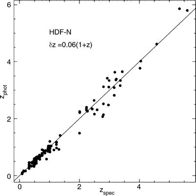
Fig. 9.8
Photometric redshift versus the
spectroscopic redshift for galaxies in the HDF-North. Photometric
data in four optical and two NIR bands have been used here. We see
how accurate photometric redshifts can be—their quality depends on
the photometric accuracy in the individual filters, the number of
filters used, the redshift and the type of the galaxy, and also on
details of the applied analysis method. Source: N. Benítez
2000, Bayesian Photometric
Redshift Estimation, ApJ 536, 571, p. 579, Fig. 5. ©AAS.
Reproduced with permission
Practical
considerations. The advantage of this method is that
multi-color photometry is much less time-consuming than
spectroscopy of galaxies. Whereas some modern spectrographs allow
one to take spectra of ∼ 1000 objects simultaneously, images taken
with wide-field cameras of ∼ 1 deg2 on 4-m class
telescopes record the fluxes of ∼ 105 galaxies in a one
hour exposure. In addition, this method can be extended to much
fainter magnitudes than are achievable for spectroscopic redshifts.
The disadvantage of the method becomes obvious when an insufficient
number of photometric bands are available, since then the
photometric redshift estimates can yield a completely wrong
z; these are often called
catastrophic outliers. One
example for the occurrence of extremely wrong redshift estimates is
provided by a break in the spectral energy distribution. Depending
of whether this break is identified as the Lyman-break or the
4000 Å-break, the resulting redshift estimates will be very
different. To break the corresponding degeneracy, a sufficiently
large number of filters spread over a broad spectral range must be
available to probe the spectral energy distribution over a wide
range in wavelengths. As a general rule, the more photometric bands
are available and the smaller the uncertainties in the measured
magnitudes, the more accurate the estimated redshift. Normally,
data from four or five photometric bands are required to obtain
useful redshift estimates. In particular, the reliability of the
photometric redshift benefits from data over a large wavelength
range, so that a combination of several optical and NIR filters is
desirable.
The successful application of this method also
depends on the type of the galaxies. As we have seen in
Sect. 6.8, early-type galaxies form a
relatively well-defined color-magnitude sequence at any redshift,
due to their old stellar populations (manifested in clusters of
galaxies in form of the red cluster sequence), so that the redshift
of this type of galaxy can be estimated very accurately from
multi-color information. However, this is only the case if the
4000 Å-break is located in between two of the applied filters. For
z ≳ 1 this is no longer the
case if only optical filters are used. Other types of galaxies show
larger variations in their spectral energy distribution, depending,
e.g., on the star formation history, as mentioned before.
Photometric redshifts are particularly useful for
statistical purposes, for instance in situations in which the exact
redshift of each individual galaxy in a sample is of little
relevance. However, by using a sufficient number of optical and NIR
filters, quite accurate redshift estimates for individual galaxies
are achievable. For example, with eight optical and NIR bands and
accurate photometry, a redshift accuracy of Δ z ∼ 0. 03(1 + z) was obtained, as demonstrated in
Fig. 9.8 by a
comparison of photometric redshifts with redshifts determined
spectroscopically for galaxies in the field of the HDF-North. If
data in additional photometric bands are available, e.g., using
filters of smaller transmission curves (‘intermediate width
filters’), the redshift accuracy can be increased even more, e.g.,
Δ z ∼ 0. 01(1 +
z) was obtained using a
total of 30 photometric bands.
9.1.3 Other few-band selection techniques
The Lyman-break technique is a special case of
the photometric redshift method; it relies on only three
photometric bands to select galaxies in a given redshift range,
whereas in general, more bands are needed to obtain reliable
redshift estimates. There are other cases where a few bands are
sufficient for a fairly reliable selection of particular kinds of
galaxies, or particular redshift regimes, some of which should be
mentioned here.
Selection
of 1. 5 ≲ z ≲ 2. 5
galaxies. The success of the
Lyman-break method is rooted in the fact that the observed colors
of star-forming galaxies in a carefully selected triplet of filters
is essentially independent on details of the star-formation
history, metallicity and other effects, due to a very strong
spectral break. This is illustrated in Fig. 9.4. The same figure also
shows that the colors of galaxies with somewhat lower redshift are
also very similar; for example, one sees that galaxies with
z ∼ 1. 8 all have
U n −
G ∼ 0 and  . At that redshift, the
Lyα-line is shortward of
the U n-band
filter, and thus a star-forming galaxy has a rather flat spectrum
across all three filters. As the redshift increases above
z ∼ 2, the Lyα-line moves into the
Un-band filter and thus increases the flux there;
however, as we have seen, a large fraction of LBGs have rather low
Lyα-flux, thus affecting
the color only marginally. For redshifts higher than ∼ 2. 5, the
break moves into the Un-band, and the objects redden in
U n −
G and move onto the same
sequence where LBGs are selected. Thus, with a single set of three
filters (and thus the same optical images), one can select galaxies
over the broad range of 1. 5 ≲ z ≲ 3. 5.
. At that redshift, the
Lyα-line is shortward of
the U n-band
filter, and thus a star-forming galaxy has a rather flat spectrum
across all three filters. As the redshift increases above
z ∼ 2, the Lyα-line moves into the
Un-band filter and thus increases the flux there;
however, as we have seen, a large fraction of LBGs have rather low
Lyα-flux, thus affecting
the color only marginally. For redshifts higher than ∼ 2. 5, the
break moves into the Un-band, and the objects redden in
U n −
G and move onto the same
sequence where LBGs are selected. Thus, with a single set of three
filters (and thus the same optical images), one can select galaxies
over the broad range of 1. 5 ≲ z ≲ 3. 5.
Fig. 9.9
Two color diagram (B − z) vs (z − K) for K-band selected galaxies of the
K20 survey in the GOODS field. Red
solid triangles and circles denote star-forming and passive
galaxies, respectively, at z ≥ 1. 4, and blue open squares correspond to
additional z ≥ 1. 4 objects
as determined from their photometric redshifts. Black solid squares are galaxies with
redshift below 1.4, and the green
asterisks are stars. Encircles symbols are galaxies detected
in X-rays. The various lines delineate regions of photometric
selection of z > 1. 4
galaxies—see text. Source: E. Daddi et al. 2004, A New Photometric Technique for the Joint
Selection of Star-forming and Passive Galaxies at
1. 4 ≲ z ≲ 2. 5, ApJ 617,
746, p. 749, Fig. 3. ©AAS. Reproduced with permission
BzK
selection. While the filter combination used for the
Lyman-break galaxies selects star-forming galaxies at high
redshift, it misses galaxies with a passive stellar population. One
has therefore investigated whether another combination of filters,
and thus different colors, may be able to identify high-redshift
passive galaxies. Indeed, such a filter set was found; the
combination of the B-, z- and K-band filters provides a successful
tool to search for galaxies with 1. 4 ≲ z ≲ 2. 5, as illustrated in
Fig. 9.9.
K-band selected galaxies with 1. 4 ≲ z ≲ 2. 5 occupy specific regions in a
B − z versus z − K color-color diagram.2 In this redshift range, the
4000 Å-break is located redward of the z-band, thus such galaxies
display a fairly red z −
K color if they are not
forming stars at a high rate. The lack of active star formation
also causes the B −
z color to be rather red,
since the B-band probes to the rest-frame UV-region of the
spectrum. Such galaxies are located in the upper right corner of
the diagram in Fig. 9.9. In case the galaxies in this redshift range
are actively forming stars, the 4000 Å-break is weaker, but instead
the B − z color is rather blue, so that these
galaxies are located in the upper left corner of the diagram. As
Fig. 9.9
shows, this selection of high-redshift galaxies is very
efficient.
The BzK-selected galaxies with active star
formation have redder colors in the rest-frame UV than the
Lyman-break galaxies which are selected based on their UV flux,
although there is a significant overlap between the two populations
in the sense that a substantial fraction of galaxies are found by
both methods. However, the most actively star-forming galaxies are
missed with the BzK-method since those show little-to-no
4000 Å-break, thus no longer have a sufficiently red z − K color, and would lie below the solid
line in Fig. 9.9.

Fig. 9.10
The evolution of (J − K) color as a function of redshift.
Solid curves show the color
for different ages of the stellar population. Dashed and dotted curves correspond to stellar
populations with continuous star formation, for different ages and
reddening. The dash-dotted
curve corresponds to a single age population formed at
z = 5. The color is redder
than  for the single-age stellar populations at z > 2. 5, and for the one formed at
z = 5, this color criterion
is satisfied for all z > 2. Source: M. Franx et
al. 2003, A Significant
Population of Red, Near-Infrared-selected High-Redshift
Galaxies, ApJ 587, L79, p. L80, Fig. 1. ©AAS. Reproduced
with permission
for the single-age stellar populations at z > 2. 5, and for the one formed at
z = 5, this color criterion
is satisfied for all z > 2. Source: M. Franx et
al. 2003, A Significant
Population of Red, Near-Infrared-selected High-Redshift
Galaxies, ApJ 587, L79, p. L80, Fig. 1. ©AAS. Reproduced
with permissionDistant red
galaxies. Another method to select high-redshift passive
galaxies is based on their rest-frame optical colors. From local
galaxies we know that the 4000 Å-break is the most prominent
feature in the spectral energy distribution of stellar populations
with no or little star formation. At redshifts 2 ≲ z ≲ 4, this break is located between
the observed J- and K-band filters; hence we expect that passive
galaxies are red in their J
− K color. As
Fig. 9.10
shows, J − K ≳ 2. 3 as soon as the redshift
increases beyond z ≳ 2.
Perhaps surprisingly, this is true even if the stellar population
is as young as 0. 25 Gyr, for which the redshift of the transition
to J − K > 2. 3 occurs at only slighter
larger redshift. Furthermore, this color selection is able to find
also galaxies with ongoing star formation, provided they also have
an old stellar population; this is due to the fact that much of the
star formation is accompanied by substantial dust obscuration. At
redshift z = 2, the J-band
corresponds to the rest-frame B-band, which is substantially
affected by extinction, leading to a red J − K color. High-redshift galaxies
selected according to J −
K > 2. 3 are called
distant red galaxies
(DRGs). The fact that there is very little overlap in the
galaxy population selected according to their UV-properties and the
DRG population immediately shows the necessity to apply several
very different selection criteria for high-redshift galaxies to
obtain a complete census of their population.
Narrow-band
selection. We mentioned the method of narrow-band selection
before. If a source has a strong emission line, and if the observed
wavelength of the emission line matches the spectral response of a
narrow-band filter, then the ratio of fluxes obtained in this
narrow-band image compared to a broad-band image would be much
larger than for other sources without a strong emission line at the
corresponding wavelength.
After a substantial population of high-redshift
galaxies were found with the Lyman Break technique, it became known
that about 60 % of these galaxies show very strong Lyα emission lines. It was then possible
to design narrow-band filters that were particularly tuned to
detect objects with strong Lyα emission lines at a particular
redshift. Several thousand Lyα emitters (LAEs) were detected with
this method, extending up to redshift z ∼ 7. These galaxies are on average
considerably fainter than LBGs, and therefore allow one to probe
the fainter end of the luminosity function of star-forming
galaxies. Their faintness, on the other hand, make more detailed
spectroscopic studies very challenging, and thus the relation of
these Lyα emitters to the
other galaxy populations at similar redshifts is not easy to
determine.
Furthermore, candidate objects detected in
narrow-band images require spectroscopic follow-up, since there are
many possible contaminants that may enter the selection. Galaxies,
and in particular AGNs, at lower redshifts can display strong
emission lines of other atomic transitions and need to be ruled out
with a spectrum. Due to the cumulative effect of the Lyα forest, a high-redshift (z ≳ 4) Lyα emitter should show essentially no
flux at shorter wavelengths, and so some of the Lyα emission-line candidates can be
rejected if continuum flux bluewards of the narrow band is
detected.
9.2 Deep views of the Universe
Very distant objects in the Universe are expected
to be exceedingly faint. Therefore, in order to find the most
distant, or earliest, objects in the Universe, very deep images of
the sky are needed to have a chance to detect them.
In order to get further out into the Universe,
astronomers use their most sensitive instruments to obtain
extremely deep sky images. The Hubble Deep Field, already discussed
briefly in Sect. 1.3.3, is perhaps the best-known
example for this. As will be discussed below, further instrumental
developments have led to even deeper observations with the HST.
Deep fields are taken also with ground-based optical and near-IR
telescopes. Although the sensitivity limit from the ground is
affected by the atmosphere, in particular at longer wavelengths,
this drawback is partly compensated by the larger field-of-view
that many ground-based instruments offer, compared to the
relatively small field-of-view of the HST. Dep field observations
are conducted also at other wavelengths, preferentially in the same
sky areas as the deep optical fields, to enable
cross-identification and thus provide additional information on the
detected sources. As we shall see, the availability of such deep
fields has allowed us to take a first look at the first 10 % of the
Universe’s life.
9.2.1 Hubble Deep Fields
The Hubble Deep
Field North. In 1995, an unprecedented observing program was
conducted with the HST. A deep image in four filters
(U300, B450, V606, and
I814) was observed with the Wide Field/Planetary Camera
2 (WFPC2) on-board HST, covering a field
of ∼ 5. 3 arcmin2, with a total exposure time of about
10 days. This resulted in the deepest sky image of that time,
displayed in Fig. 1.37. The observed field was
carefully selected such that it did not contain any bright sources.
Furthermore, the position of the field was chosen such that the HST
was able to continually point into this direction, a criterion
excluding all but two relatively small regions on the sky, due to
the low HST orbit around the Earth. Another special feature of this
program was that the data became public right after reduction, less
than a month after the final exposures had been taken. Astronomers
worldwide immediately had the opportunity to scientifically exploit
these data and to compare them with data at other frequency ranges
or to perform their own follow-up observations. Such a rapid and
wide release was uncommon at that time, but is now seen more
frequently. Rarely has a single data set inspired and motivated a
large community of astronomers as much as the Hubble Deep Field (HDF) did (after
another HDF was observed in the Southern sky—see below—the original
HDF was called HDF North, or HDFN).
Follow-up observations of the HDF were made in
nearly all accessible wavelength ranges, so that it became the
best-observed region of the extragalactic sky. Within a few years,
more than ∼ 3000 galaxies, 6 X-ray sources, 16 radio sources, and
fewer than 20 Galactic stars were detected in the HDF, and
redshifts were determined spectroscopically for more than 150
galaxies in this field, with about 30 at z > 2. Never before could galaxy
counts be conducted to magnitudes as faint as it became possible in
the HDF (see Fig. 9.11); several hundred galaxies per square
arcminute could be photometrically analyzed in this field.
Detailed spectroscopic follow-up observations
were conducted by several groups, through which the HDF became,
among other things, a calibration field for photometric redshifts
(see, for instance, Fig. 9.8). Most galaxies in the HDF are far too faint
to be analyzed spectroscopically, so that one often has to rely on
photometric redshifts.

Fig. 9.11
Galaxy counts from the HDF and other
surveys in four photometric bands: U, B, I, and K. Solid symbols are from the HDF,
open symbols from various
ground-based observations. The curves represent predictions from
models in which the spectral energy distribution of the galaxies
does not evolve—the counts lie significantly above these so-called
non-evolution models: clearly, the galaxy population must be
evolving. Note that the counts in the different color filters are
shifted by a factor 10 each, simply for display purposes. Source:
H. Ferguson et al. 2000, The Hubble Deep Fields, ARA&A 38,
667, Fig. 4. Reprinted, with permission, from the Annual Review of Astronomy &
Astrophysics, Volume 38 ©2000 by Annual Reviews www.annualreviews.org
HDFS and the
Hubble Ultra Deep Field. Later, in 1998, a second HDF was
observed, this time in the southern sky. In contrast to the HDFN,
which had been chosen to be as empty as possible, the HDFS contains
a QSO. Its absorption line spectrum can be compared with the
galaxies found in the HDFS, by which one hopes to obtain
information on the relation between QSO absorption lines and
galaxies. In addition to the WFPC2 camera, the HDFS was
simultaneously observed with the cameras STIS (51″ × 51″
field-of-view, where the CLEAR ‘filter’ was used, which has a very
broad spectral sensitivity; in total, STIS is considerably more
sensitive than WFPC2) and NICMOS (a NIR camera with a maximum
field-of-view of 51″ × 51″) which had both been installed in the
meantime. Nevertheless, the overall impact of the HDFS was smaller
than that of the HDFN; one reason for this may be that the
requirement of the presence of a QSO, combined with the need for a
field in the continuous viewing zone of HST, led to a field close
to several very bright Galactic stars. This circumstance makes
photometric observations from the ground very difficult, e.g., due
to stray-light.
One of the immediate results from the HDF was the
finding that the morphology of faint galaxies is quite different
from those in the nearby Universe. Locally, most luminous galaxies
fit into the morphological Hubble sequence of galaxies. This ceases
to be the case for high-redshift galaxies. In fact, galaxies at
z ∼ 2 are much more compact
than local luminous galaxies, they show irregular light
distributions and do not resemble any of the Hubble sequence
morphologies. By redshifts z ∼ 1, the Hubble sequence seems to
have been partly established.
In 2002, an additional camera was installed
on-board HST. The Advanced Camera
for Surveys (ACS) has, with its side length of
3.′4, a field-of-view about twice as large as WFPC2,
and with half the pixel size (0.″05) it better matches
the diffraction-limited angular resolution of HST. Therefore, ACS
is a substantially more powerful camera than WFPC2 and is, in
particular, best suited for surveys. With the Hubble Ultra Deep Field (HUDF), the
deepest image of the sky was observed and published in 2004 (see
Fig. 9.12).
The HUDF is, in all four filters, deeper by about one magnitude
than the HDF, reaching a magnitude limit of m AB ≈ 29. The depth of the
ACS images in combination with the relatively red filters that are
available provides us with an opportunity to identify drop-out
candidates out to redshifts z ∼ 6; quite a number of such
candidates have already been verified spectroscopically.
Lyman-break galaxies at z ∼ 6 seem to have stellar populations
with masses and lifetimes comparable to those at z ∼ 3. This implies that at a time when
the Universe was 1 Gyr old, a stellar population with mass ∼ 3 ×
1010 M
⊙ and age of a few hundred million years (as indicated
by the observed 4000 Å break) was already in place. This, together
with the apparently high metallicity of these sources, is thus an
indication of how quickly the early Universe evolved. The
z ∼ 6 galaxies are very
compact, with half-light radii of ∼ 1 kpc, and thus differ
substantially from the galaxy population known in the
lower-redshift Universe.
Half of the HUDF was also imaged by the near-IR
NICMOS camera onboard HST, but only after the installment

Fig. 9.12
The Hubble Ultra Deep Field, a field
of ∼ 3.′4 × 3.′4 observed by the ACS
camera. The limiting magnitude up to which sources are detected in
this image is about one magnitude fainter than in the HDF. More
than 10 000 galaxies are visible in the image, many of them at
redshifts z ≥ 5. Credit:
NASA, ESA, S. Beckwith/Space Telescope Science Institute, and
the HUDF Team
of the Wide-Field Camera 3 (WFC3) on HST, with
a near-IR channel and a much larger field-of-view and much better
sensitivity than NICMOS, could the HUDF be imaged to comparable
sensitivity levels in the NIR as in the optical. WFC3 mapped the
HUDF in three NIR bands, Y, J and H, down to a limiting magnitude
of m AB ≈ 28. 5.
These long wavelengths allowed the systematic search for
Lyman-break galaxies at redshifts beyond 6, as will be discussed
below.
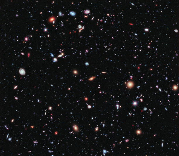
Fig. 9.13
The Hubble eXtreme Deep Field (XDF) covers
an area of 2.′3 × 2′, centered on the HUDF, and was
composed with HST observations spread over many years. The total
exposure time amounts to about 2 million seconds, or 22 days. This
color composite was made from data in eight different optical and
NIR bands, taken with the ACS and WFC3/IR instruments. Credit:
NASA, ESA, G. Illingworth, D. Magee, and P. Oesch
(University of California, Santa Cruz), R. Bouwens (Leiden
University), and the HUDF09 Team
In September 2012, the deepest view of the
Universe ever taken was released: the eXtreme Deep Field (XDF), shown in
Fig. 9.13. It
covers about 4. 7 arcmin2 in nine optical and NIR
filters, reaching a limiting magnitude of m AB ≈ 30.
Further deep-field
projects with HST: GOODS, GEMS, COSMOS. The great scientific
harvest from the deep HST images, particularly in combination with
data from other telescopes and the readiness to make such data
available to the scientific community for multi-frequency analysis,
provided the motivation for additional HST surveys. The GOODS
(Great Observatories Origins Deep Surveys) project is a joint
observational campaign of several observatories, centering on two
fields of ∼ 16′ × 10′ size each that have been observed by the ACS
camera at several epochs between 2003 and 2005. One of these two
regions (GOODS-North) contains the HDFN, the other a field that
became known as the Chandra Deep Field South (CDFS), also
containing the HUDF. The Chandra satellite observed both GOODS
fields with a total exposure time of ∼ 2 × 10⁶ s and ∼ 4
× 106 s, corresponding to about 24 and 48 days,
respectively. Also, the Spitzer observatory took long exposures of
these two fields, and several ground-based observatories are
involved in this survey, for instance by contributing an ultra-deep
wide-field image ( ∼ 30′ × 30′) centered on the Chandra Deep Field
South and NIR images in the K-band. The data themselves and the
data products (like object catalogs, color information, etc.) are
all publicly available and have led to a large number of scientific
results.
The multi-wavelength approach by GOODS yields an
unprecedented view of the high-redshift Universe. Although these
studies and scientific analysis are ongoing (at the time of
writing), quite a large number of very high-redshift (z ≳ 5–6) galaxies were discovered and
studied: a sample of more than 500 I-band drop-out candidates was
obtained from deep ACS/HST images.
Even larger surveys were conducted with the HST,
including the Galaxy Evolution from Morphology and SEDs (GEMS)
survey, covering a field of 30′ × 30′ centered on the CDFS mapped
in two filters. For this field, full coverage with a 17-band (5
broad bands, and 12 intermediate width bands) optical imaging
survey (COMBO17) is available. The largest contiguous field imaged
with the angular resolution of HST is the ∼ 2 deg2
COSMOS survey. This sky area was also imaged with other space-based
(Spitzer, GALEX, XMM-Newton, Chandra) and ground-based (Subaru,
VLA, VLT, UKIRT and others) observatories. Its large field enables
the study of the large-scale galaxy and AGN distribution at high
redshifts. The broad wavelength coverage from the radio to the
X-ray regime, renders the COSMOS field a treasure for observational
cosmology for years to come. As discussed in Sect. 8.4, the COSMOS field was used for a
detailed cosmic shear analysis, where the broad wavelength coverage
helped enormously to determine accurate photometric redshifts of
the source galaxies.
9.2.2 Deep fields in other wavebands
Deep fields have been observed in many other
frequency ranges, and as mentioned before, they are often taken on
the same sky areas to allow for multi-frequency studies of the
sources. We mention here the Chandra Deep Fields, one in the North
(CDFN) in the direction of the HDFN, the other in the South (CDFS,
see Fig. 9.14) in the direction of the HUDF, with a
total exposure time of two and four million seconds,
respectively.
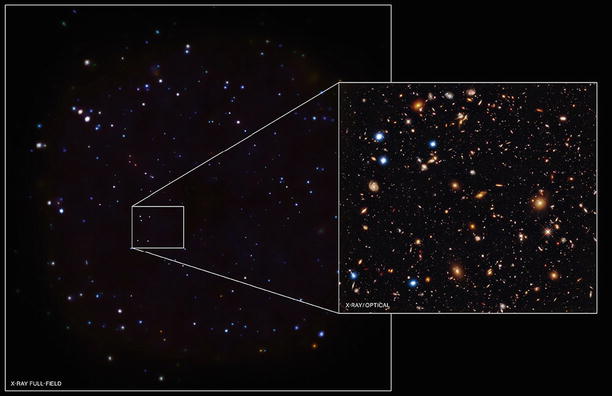
Fig. 9.14
The Chandra Deep Field South (CDFS), an
X-ray image of a ∼ 450 arcmin2 field with a total
exposure time of 4 × 10⁶ s. This is the deepest image
ever taken of the X-ray sky. The right panel shows a color composite
image taken with HST. Credit: X-ray: NASA/CXC/U.Hawaii/E.Treister
et al.; optical: NASA/STScI/S.Beckwith et al.)
Fig. 9.15
Cumulative compact source counts
N( > S) as obtained from the CDFS (see
Fig. 9.14),
in the soft (a) and hard
(b) energy bands, split
according to source populations: AGNs (blue), galaxies (red) and Galactic stars (green). Source: B.D. Lehmer et
al. 2012, The 4 Ms Chandra
Deep Field-South Number Counts Apportioned by Source Class:
Pervasive Active Galactic Nuclei and the Ascent of Normal
Galaxies, ApJ 752:46, p. 7, Fig. 5. ©AAS. Reproduced with
permission
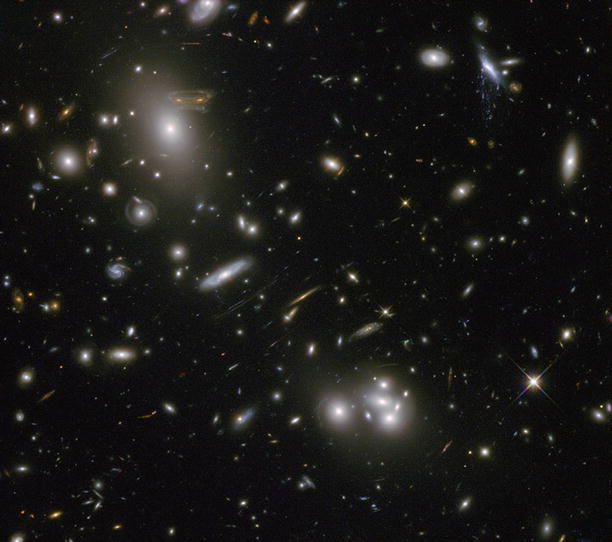
Fig. 9.16
HST images of the lensing cluster Abell 68
magnifying many faint background galaxies. Several z > 5 candidates are found in this
field, at least one of them spectroscopically verified. Credit:
NASA, ESA, and the Hubble Heritage/ESA-Hubble Collaboration,
Acknowledgment: N. Rose

Fig. 9.17
The image on the left was taken by the Hubble
Space Telescope. It shows the cluster of galaxies MS 1512+36, which
has a redshift of z = 0. 37. To the right, and slightly
above the central cluster galaxy, an extended and apparently very
blue object is seen, marked by an arrow. This source is not physically
associated with the cluster but is a background galaxy at a
redshift of z = 2. 72. With
this HST image it was proved that this galaxy is strongly lensed by
the cluster and, by means of this, magnified by a factor of ∼ 30.
Due to the magnification, this Lyman-break galaxy is the brightest
normal galaxy at redshift z ∼ 3, a fact that can be profitably
used for a detailed spectroscopic analysis. On the right, a small section from a
high-resolution VLT spectrum of this galaxy is shown. The
Lyα transition of the
galaxy is located at λ = 4530 Å, visible as a broad
absorption line. Absorption lines at shorter wavelengths originate
from the Lyα-forest along
the line-of-sight (indicated by short vertical lines) or by metal lines
from the galaxy itself (indicated by arrows). Credit: Left: S. Seitz, HST; corresponding
research article: S. Seitz et al. 1998, The z = 2. 72 galaxy cB58: a gravitational fold arc lensed
by the cluster MS1512+36, MNRAS 298, 945. Right: European Southern
Observatory
With the extremely faint limiting flux of the
CDFS, the source density on the sky reaches more than
104 deg−2, which is comparable to the source
density seen in rather shallow optical imaging, like the SDSS
images. However, the mean redshift of the X-ray sources is
considerably higher than that of the optical sources, due to the
large fraction of AGNs. As we can see from Fig. 9.15, the X-ray
population of compact sources in ultra-deep X-images is composed of
three components. By far dominating is the population of AGNs,
whose number counts exhibit the shape of a broken power law—steep
at the bright end, flatter at the low-flux end. For high fluxes,
they follow approximately the Euclidean slope,  , whereas
at fluxes below the breakpoint at
, whereas
at fluxes below the breakpoint at  ,
one finds
,
one finds  for the
soft band, and even slightly flatter in the hard band. Going to
fainter X-ray fluxes, the fraction of obscured AGNs at high
redshifts increases.
for the
soft band, and even slightly flatter in the hard band. Going to
fainter X-ray fluxes, the fraction of obscured AGNs at high
redshifts increases.
, whereas
at fluxes below the breakpoint at ,
one finds for the
soft band, and even slightly flatter in the hard band. Going to
fainter X-ray fluxes, the fraction of obscured AGNs at high
redshifts increases.Approaching the fainter flux levels, the
population of normal galaxies becomes increasingly important. At
the limiting flux of the CDFS, they constitute almost 50 % of the
source population. They are mainly late-type star-forming galaxies,
with the X-ray emission mostly due to X-ray binaries. Early-type
galaxies contribute just a small fraction of ∼ 10 % to the galaxy
counts, where their X-ray emission is a due to a combination of
X-ray binaries and hot gas.
9.2.3 Natural telescopes
Galaxies at high redshift are faint and therefore
difficult to observe spectroscopically. For this reason, the
brightest galaxies are preferentially selected (for detailed
examination), i.e., basically those which are the most luminous
ones at a particular z—resulting in undesired, but hardly
avoidable selection effects. For example, those Lyman-break
galaxies at z ∼ 3 for which
the redshift is verified spectroscopically are typically located at
the bright end of the LBG luminosity function. The sensitivity of
our telescopes is insufficient in most cases to spectroscopically
analyze a rather more typical galaxy at z ∼ 3.
The magnification by gravitational lenses can
substantially boost the apparent magnitude of sources;
gravitational lenses can thus act as natural (and inexpensive!)
telescopes. The most prominent examples are the arcs in clusters of
galaxies: many of them have a very high redshift, are magnified by
a factor ≳ 5, and hence are brighter by about ≳ 1. 5 mag than they
would be without the lens effect (see Fig. 9.16).3 In addition to boosting the
observable fluxes, the gravitational lens effect yields a spatial
magnification of the sources: the sources appear larger than they
really are, thus increasing the effective angular resolution with
which they can be observed.
Lyman-break
galaxies at z ∼ 3.
An extreme first example of this effect is represented by the
galaxy cB58 at z = 2. 72,
which is displayed in Fig. 9.17. It was discovered in the background of a
galaxy cluster and is magnified by a factor ∼ 30. Hence, it appears
brighter than a typical Lyman-break galaxy by more than three
magnitudes. For this reason, one of the most detailed spectra of
all galaxies at z ∼ 3 was
taken of this particular source. Several more such examples were
found subsequently, including the so-called Cosmic Eye, a
Lyman-break galaxy at z = 3. 07, shown in Fig. 9.18. The typical
magnification of these lensed LBGs is μ ∼ 30.
Further
examples. Furthermore, at least two highly magnified
Lyα emitters (LAEs) at
z ≈ 5 were found. Whereas
the study of LAEs is usually hampered by the faint continuum, the
strong magnification (μ > 10 in these two systems) enables
an investigation of the underlying stellar population from
broad-band photometry. One of these two systems has an estimated
stellar mass of ≲ 108 M ⊙, one of the lowest mass
systems found so far at high redshifts. Thanks to the increased
effective angular resolution provided by gravitational lensing
magnification, a spatially resolved view of the star-forming
regions in a z = 2. 33
sub-millimeter galaxy was obtained. The observations are compatible
with the picture that star formation in this object occurs in the
cores of giant molecular clouds, as in the local Universe, but
these regions are ∼ 100 times larger than local star-forming
sites.
Fig. 9.18
The Cosmic Eye is a Lyman-break galaxy at
z = 3. 07, gravitationally
lensed by an early-type galaxy at z = 0. 73, which itself is located in
the background of a massive galaxy cluster at z = 0. 33. The angular extent of the
arc systems is ∼ 3″; this large image splitting is due to the
combined lensing effect of the main lens galaxy and the foreground
cluster, which magnify the source galaxy by a factor μ ∼ 30. Hence, this image is almost 4
magnitudes brighter than the unlensed source. Credit: D.P. Stark,
HST

Fig. 9.19
A section of the galaxy cluster
Abell 2218 (z = 0. 175), observed with the HST in
four different filters. This region was selected because the
magnification by the gravitational lens effect for sources at high
redshift is expected to be very large here. This fact has been
established by a detailed mass model of this cluster which could be
constructed from the geometrical constraints provided by the
numerous arcs and multiple images (Fig. 6.51). The red lines denote the critical curves of
this lens for source redshifts of z = 5, 6.5, and 7. A double image of an
extended source is clearly visible in the NIR image (on the right); this double image was
not detected at shorter wavelengths—the expected position is marked
by two ellipses in the two images on the left. The direction of the local
shear, i.e., of the expected image distortion, is plotted in the
second image from the
right; the observed elongation of the two images a and b is
compatible with the shear field from the lens model. Together with
the photometry of these two images, a redshift between z = 6. 8 and z = 7 was derived for the source of
this double image. Source: J.-P. Kneib et al. 2004,
A Probable z ∼ 7
Galaxy Strongly Lensed by the Rich
Cluster A2218: Exploring the Dark Ages, ApJ 607, 697,
p. 698, Fig. 1. ©AAS. Reproduced with permission
Apparently extreme
sources. One can argue that there is a high probability that
the flux of the apparently most luminous sources from a particular
source population is magnified by lensing. The apparently most
luminous IRAS galaxy, F10214+47, is magnified by a factor ∼ 50 by
the lens effect of a foreground galaxy, where the exact value of
the magnification depends on the wavelength, since the intrinsic
structure and size of the source is wavelength-dependent—hence the
magnification is differential. Other examples are the QSOs
B1422+231 and APM 08279+5255, which are among the brightest QSOs
despite their high redshifts; hence, they belong to the apparently
most luminous sources in the Universe. In both cases, multiple
images of the QSOs were discovered, verifying the action of the
lens effect. Their magnification, and therefore their brightness,
renders these sources preferred objects for QSO absorption line
spectroscopy (see Fig. 5.55). The Lyman-break galaxy cB58
mentioned previously is another example, and we will see below that
the most luminous sub-millimeter sources are gravitationally
lensed.
Employing natural
telescopes. Most of the examples of highly magnified sources
mentioned before were found serendipitously. However, the
magnification effect can also be utilized deliberately, by
searching for high-redshift sources in regions which are known to
produce strong magnification effects, i.e., fields around clusters
of galaxies: for a massive cluster, one knows that distant sources
located behind the cluster center are substantially magnified. It
is therefore not surprising that some of the most distant galaxies
known have been detected in systematic searches for drop-out
galaxies near the centers of massive clusters. One example of this
is shown in Fig. 9.19, where a galaxy at z ∼ 7 is doubly imaged by the cluster
Abell 2218 (see Fig. 6.51), and by means of this it is
magnified by a factor ∼ 25.
The CLASH and HLS
surveys. In order to fully exploit the power of natural
telescopes, a large treasury program was carried out with HST,
imaging 25 massive clusters with 16 filters of the ACS and WFC3/IR
instruments. This CLASH (Cluster Lensing And Supernova survey with
Hubble) survey is designed to obtain accurate spectral energy
distributions of very faint galaxies in the cluster fields.
Furthermore, the data will allow high-quality strong and weak
lensing analysis of these clusters, and many results are already
available at the time of writing. The observing strategy with
multiple visits per cluster field also enables the detection of
supernovae, either of cluster galaxies, or gravitationally lensed
background supernovae.

Fig. 9.20
Left
panel: Similar to Fig. 9.4, evolutionary tracks of stellar populations
in a near-IR color-color diagram are shown, for different galaxy
types. The two blue tracks
correspond to starburst galaxies, and they differ in the assumed
slope β of the continuum UV
spectrum. The corresponding redshifts are written near the tracks.
Black points show the
near-IR colors of galaxies detected at optical wavelengths in the
HUDF. The red squares with
error bars correspond to five galaxies which are clearly detected
in at least two near-IR bands, but with no detection in any optical
filter—see the right panel,
where cut-outs around these sources in the HUDF optical and WFC3/IR
images are shown. These were selected by the color criteria
indicated by the grey
region. Source: R.J. Bouwens et al. 2010, Discovery of z ∼ 8 Galaxies in the Hubble Ultra Deep Field from
Ultra-Deep WFC3/IR Observations, ApJ 709, L133, p. L135,
Figs. 1, 2, 3. ©AAS. Reproduced with permission
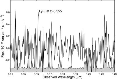
Fig. 9.21
Spectrum of the galaxy UDFy-38135539, for
which multiband images are shown in Fig. 9.20, obtained with
integral field spectrograph SINFONI at the VLT. The grey band at the bottom shows the shape
of the night-sky spectrum. The total integration time for this
spectrum was 15 h. The Ly α
line marked at λ = 11 616 Å
is broader than the instrumental resolution, and is detected
with ∼ 6σ significance.
Source: M.D. Lehnert et al. 2010, Spectroscopic confirmation of a galaxy at
redshift z=8.6, Nature 467, 940, Fig. 1. Reprinted by
permission of Macmillan Publishers Ltd: Nature, ©2010
In a similar spirit, the Herschel Lensing Survey
(HLS) targeted 44 massive clusters, in order to find magnified
far-IR sources; some of the results from this survey will be
discussed in Sect. 9.3.3 below.
9.2.4 Towards the dark ages
We have seen that in order to apply the
Lyman-break technique, one needs images in three filters, one on
the blue side of the Lyman break, and two on the red side. These
two redder filters are required to demonstrate that these galaxies
have a rather flat spectrum for wavelengths longer than the break,
i.e., that they are indeed actively star forming, to minimize the
possibility that the source is simply a very red one and drops out
of the shorter wavelength filter just for this reason. Therefore,
the application of the Lyman-break method on deep optical images is
restricted to redshifts of z ≲ 5. In order to move towards higher
redshifts, images in the near-IR are required.
Combining the images of the HUDF with deep NIR
imaging from NICMOS and with ground-based telescopes, the redshift
z ∼ 6 barrier could be
overcome, by searching for i-band dropouts. Many of these were
found, and several of the brighter ones were spectroscopically
confirmed. Furthermore, ultra-deep optical and NIR imaging from the
ground, covering larger sky areas than possible with the HST, have
brought large harvest in selecting z ∼ 6 galaxies using the Lyman-break
technique. Currently, more than 30 galaxies are known with
spectroscopic redshifts between 6 and 6.5.

Fig. 9.22
The galaxy cluster MACS J0647+7015
(z = 0. 591) as observed by
the HST in the framework of the CLASH survey. The image is a
multi-band composite, based on images in 13 different bands. The
three small panels on the left of
the top image are zooms of a multiply imaged source. The
bottom panel shows the
critical curves of the lens model for this cluster, for sources at
different redshifts of z = 2. 0 (cyan), z = 3. 5 (green) and z = 11. 0 (red). Several strongly lensed images
are identified and labeled, where the number of the label identify
the same source, and the lower-case letter are assigned to the
multiple images. From the lens model of the cluster, which yields
an estimate of the magnification μ ≈ 7 for the brightest image, and the
multi-band photometry, a likely redshift of z ∼ 10. 7 is estimated for the source.
Top: Credit: NASA, ESA, M.
Postman and D. Coe (STScI), and the CLASH Team. Bottom: Source: D. Coe et
al. 2013, CLASH: Three
Strongly Lensed Images of a Candidate z ≈ 11 Galaxy, ApJ
762, 32, p 3, Fig. 1. ©AAS. Reproduced with permission
As we saw before, QSOs at these redshifts have
essentially no flux shortward of the Lyα emission line, i.e., the
intergalactic medium at z ∼ 6 is sufficiently neutral to absorb
almost all UV-photons. This could mean that we are approaching the
redshift of reionization of the Universe, and it is not immediately
obvious that one may expect a substantial population of
higher-redshift objects. On the other hand, the photons needed for
reionizing the Universe must come from the first galaxies formed,
and these must occur at even higher redshifts. In addition, since
the first results from WMAP, we have known that the redshift of
reionization is substantially higher than z = 6, with the Planck CMB results
estimating this redshift to be at z ∼ 10. Thus, searching for
higher-redshift sources is a highly valuable scientific aim, in
order to understand the early stages of the evolution of
galaxies.
Once at z ∼ 7, the Lyα line is at λ ∼ 1 μm, and hence one needs at least
two NIR images, plus a very deep optical image in the z-band, in order to find LBG candidates
at these redshifts. As discussed above, the latest camera onboard
HST, the WFC3, has a sensitive near-IR channel, and its mapping of
the HUDF provided an excellent data set for this purpose. Together
with less deep, but larger-area imaging by WFC3 over the GOODS
field, some 100 candidates at z ∼ 7, and more than 50 at z ∼ 8 have been found (see
Fig. 9.20 for
several z ∼ 8 candidates).
Spectroscopic verification of these sources, however, is very
challenging, since now very sensitive near-IR spectroscopy is
needed.
For one of the high-z candidates in Fig. 9.20, the detection of a
spectral line in a deep NIR spectrum was claimed—see
Fig. 9.21—yielding a redshift of z = 8. 55. Whereas the redshift is
based on a single emission line, the identification of this line as
Lyα is considered to be
secure, since the HST photometry shown in Fig. 9.20 rules out all other
redshift, except a low-probability alternative at z ∼ 2. In this case, the emission line
would be [Oii], which is
a doublet. This doublet would have been clearly resolved in the
spectrum and can safely be ruled out. Thus, if the emission line in
Fig. 9.21 is
real, this galaxy is the highest-redshift spectroscopically
confirmed galaxy yet found. However, reobservation of the same
source with two other NIR spectrographs failed to reproduce the
emission line. Whether or not this galaxy is at z = 8. 55 thus remains an open issue,
but this example impressively illustrates the difficulty of
securing redshifts for z ≳ 7 galaxies. We also need to keep in
mind that many LBGs at lower redshift do not show a Lyα emission line; no spectroscopic
redshift of analogs of such sources at high redshifts can be
obtained with current telescopes.
Employing natural telescopes, the hunt for even
higher-redshift sources becomes promising. The cluster MACS
J0647+7015 shown in Fig. 9.22 is a target of the CLASH survey, and thus
has been imaged with HST in many different filters. One of the
multiply-imaged sources in this cluster is a J-band drop-out; its
spectral energy distribution puts it at a redshift z ∼ 11. Such a high redshift is also
supported by the lensing geometry and the location of the three
images. Whereas no spectroscopic confirmation of this high redshift
is available up to now, the next generation space telescope JWST
(see Chap. 11) will probably be able to confirm
(or not) this redshift estimate.
On the other hand, the narrow-band selection of
high-z sources is more
promising in this respect. Although there are many contaminating
sources—emission line objects at lower redshifts—a clear detection
of a source through the narrow-band technique at least yields a
good indication that the source has an emission line at that
wavelength, and thus spectroscopy is promising.
The wavelengths of the narrow-band filters are
best chosen as to minimize the sky brightness. This then defines
preferred spectral windows, which in turn define the redshifts of
the Lyα emitting galaxies
that can be detected with this technique. By far the most
productive telescope in this respect is Subaru, due to its unique
combination of aperture and field-of-view of its Suprime-Cam
camera. Specifically designed narrow-band filters for the highest
redshifts target LAEs at z ∼ 5. 7, 6.6, 7.0 and 7.3. Many
hundreds of LAEs were found with this techniques, including several
dozens spectroscopically confirmed at redshift z ≳ 6. 6. The redshift record holder
are galaxies at z = 6. 96
and z = 7. 213.

Fig. 9.23
Two high-redshift galaxy candidates,
selected by the Lyman-break technique from deep HST fields. The
data points with error bars are flux measurements from the HST
data, complemented by MIR data from Spitzer. The small arrows indicated upper limits to
the flux in these bands. The inserts show the figure-of-merit
function χ 2 as
a function of redshift. The thick
blue line in each panel shows the best fitting spectral
energy distribution for a high-redshift galaxy, yielding
z ∼ 6. 65 and z = 6. 96 for the upper and lower
galaxy, respectively, corresponding to the minimum of the
χ 2 function. A
second spectral fit can be found when assuming a lower redshift,
shown by the dotted red
curves. In the upper
panel, this fit is indeed almost acceptable, though the
high-z fit is considerably
better—the corresponding χ
2-values as a function of redshift is shown in the
inset, and rules out the
low-redshift solution with very high confidence. The lower-redshift
fit shown in the bottom
panel can be rejected fully; this z ∼ 7 estimate seems to be very robust.
Source: R.J. McLure et al. 2011, A robust sample of galaxies at redshifts 6.0
< z < 8.7: stellar populations, star formation rates and
stellar masses, MNRAS 418, 2074, Fig. 2. Reproduced by
permission of Oxford University Press on behalf of the Royal
Astronomical Society
Fig. 9.24
The spectrum of the QSO ULAS J1120+0641 at
z = 7. 085 is shown in
black, superposed on a
composite spectrum of lower-redshift QSOs. Several emission lines
redwards of the Lyman-α
line are marked. The two spectra are in very good agreement, except
of course for rest wavelengths smaller than the Lyman-α line, due to exceedingly strong
absorption by the Lyα
forest. However, the Civ
line of ULAS J1120+0641 seems to be significantly blueshifted,
relative to the composite spectrum. Source: D.J. Mortlock et
al. 2011, A luminous quasar
at a redshift of z = 7.085, Nature 474, 616, Fig. 1.
Reprinted by permission of Macmillan Publishers Ltd: Nature,
©2011
In many cases photometric redshifts may be the
only method for obtaining redshift information, until more powerful
telescopes come into operation. As mentioned before, photometric
redshifts are the more reliable the more bands are available, and
the better the photometric accuracy is. Deep fields like the GOODS
field are therefore best suited for photo-z studies of high-redshift galaxies,
owing to the broad wavelength coverage and their depth. In
Fig. 9.23,
two galaxies selected by the Lyman-break technique are shown, with
optical, NIR and MIR observations available from HST and Spitzer.
In both cases, the best-fitting high-redshift and low-redshift
spectral energy distributions are shown, and in both cases, the
low-redshift fit is very much worse than the high-z one, so that a low redshift can be
ruled out with very high confidence in both cases. This
photo-z technique has
yielded substantial samples of z ≲ 8 galaxies, which form a rather
robust base for statistical studies of the high-z galaxy population.
The highest
redshift QSO. Whereas over most of the past ∼ 50 years QSOs
were the redshift record holders, this is currently no longer the
case: independent of whether the galaxy shown in Fig. 9.21 is indeed at
z = 8. 55, the
photo-z of several galaxies
are sufficiently robust to place them at z > 7. Concerning QSOs, the SDSS has
discovered several z ∼ 6
objects, with the highest redshift one at z = 6. 42 (see Fig. 9.1). This was for many
years the record holder; only recently, a QSO with z > 7 was found, whose spectrum is
shown in Fig. 9.24. It was found with a color selection,
based on optical and near-IR photometry. The spectrum clearly
confirms its high redshift of z = 7. 085, based on several emission
lines. Its high luminosity of ∼ 6 × 10¹³ L ⊙ implies a very massive
black hole with mass M ∼ 2
× 109 M
⊙, as estimated from the line width of the
Mgii emission line in
combination with the luminosity. This large SMBH mass had to be
assembled within the first 800 million years of the Universe. This
strengthens the constraints on rapid black hole formation, relative
to the previously discovered QSOs with redshifts z ≲ 6. 4.4
9.3 New types of galaxies
The Lyman-break galaxies discussed above are not
the only galaxies that are expected to exist at high redshifts. We
have argued that LBGs are galaxies with strong star formation.
Moreover, the UV radiation from their newly-born hot stars must be
able to escape from the galaxies. From observations in the local
Universe we know, however, that a large fraction of star formation
is hidden from our direct view when the star formation region is
enveloped by dust. The latter is heated by absorbing the UV
radiation, and re-emits this energy in the form of thermal
radiation in the FIR domain of the spectrum. At high redshifts such
galaxies would certainly not be detected by the Lyman-break
method.
Instrumental developments opened up new
wavelength regimes which yield access to other types of galaxies.
Two of these will be described in more detail here: EROs (Extremely
Red Objects) and sub-millimeter sources. But before we discuss
these objects, we will first investigate starburst galaxies in the
relatively local Universe.
Fig. 9.25
The Antennae galaxies. On the left, the ‘true’ optical colors
are shown, whereas in the right-hand image the reddish color shows Hα emission. This pair of merging
galaxies (also see Figs. 1.16 and 3.6 for other examples of merging
galaxies) is forming an enormous number of young stars. Both the UV
emission (bluish in the left
image) and the Hα
radiation (reddish in the right
image) are considered indicators of star formation. The
individual knots of bright emission are not single stars but star
clusters with typically 105 M ⊙; however, it is also
possible to resolve individual stars (red and blue supergiants) in
these galaxies. Source: B.C. Whitmore et al. 1999,
The Luminosity Function of Young
Star Clusters in “the Antennae” Galaxies (NGC 4038-4039), AJ
118, 1551, p. 1556, 1557, Figs. 3, 4. ©AAS. Reproduced with
permission
9.3.1 Starburst galaxies
One class of galaxies, the so-called starburst galaxies, is characterized by
a strongly enhanced star-formation rate, compared to normal
galaxies. Whereas our Milky Way is forming stars with a rate
of ∼ 3M ⊙∕yr,
the star-formation rate in starburst galaxies can be larger by a
factor of more than a hundred. Dust heated by hot stars radiates in
the FIR, rendering starbursts very strong FIR emitters. Many of
them were discovered by the IRAS satellite (‘IRAS galaxies’) ; they
are also called ULIRGs (Ultra Luminous InfraRed Galaxies).
The reason for this strongly enhanced star
formation is presumably the interaction with other galaxies or the
result of merger processes, an impressive example of which is the
merging galaxy pair known as the ‘Antennae’ (see Fig. 9.25). In this system,
stars and star clusters are currently being produced in very large
numbers. The images show a large number of star clusters with a
characteristic mass of 105 M ⊙, some of which are
spatially resolved by the HST. Furthermore, particularly luminous
individual stars (supergiants) are also identified. The ages of the
stars and star clusters span a wide range and depend on the
position within the galaxies. For instance, the age of the
predominant population is about 5–10 Myr, with a tendency for the
youngest stars to be located in the vicinity of strong dust
absorption. However, stellar populations with an age of 100 and
500 Myr, respectively, have also been discovered; the latter
presumably originates from the time of the first encounter of these
two galaxies, which then led to the ejection of the tidal tails.
This seems to be a common phenomenon; for example, in the starburst
galaxy Arp 220 (see Fig. 1.15) one also finds star clusters
of a young population with age ≲ 107 yr, as well as
older ones with age ∼ 3 × 10⁸ yr. It thus seems that
during the merging process several massive bursts of star-cluster
formation are triggered.

Fig. 9.26
The Antennae galaxies: In the left panel, superposed on the optical
HST image are contours of infrared emission at 15 μm, measured by
the ISO satellite. The right
panel shows a composite: X-ray emission as observed by
Chandra shown in blue, and
the 8 μm map obtained by
Spitzer (red), is
superposed on an optical three-band composite image from HST. The
strongest IR emission originates in optically dark regions. A large
fraction of the star formation in this galaxy pair is not visible
on optical images, because it is hidden by dust absorption. Note
that the orientation in the right
panel differs from that of the other images of the Antennae,
as it was taken with the HST at a different orientation angle.
Credit: Left: Canadian Astronomy and Astrophysics in the
21st Century, Courtesy Christine Wilson, McMaster
University. Right:
NASA/CXC/SAO/JPL-Caltech/STScI
It was shown by the ISO satellite that the most
active regions of star formation are not visible on optical images,
since they are completely enshrouded by dust (left panel in
Fig. 9.26). A
map at 8 μm obtained by the Spitzer Space Observatory
(Fig. 9.26,
right panel) shows the hot dust heated by young stars, where this
IR emission is clearly anti-correlated with the optical radiation.
Indeed, the mid-infrared emission is strongest in the region
between these two colliding galaxies; apparently, this is the
location where the current star formation is most intense. Maps of
the CO emission also show that these regions contain a large
reservoir of molecular gas. Furthermore, the large-scale X-ray
radiation in this galaxy collision shows the efficiency with which
gas is heated to high temperatures by the supernova events that
accompany massive star formation, with a corresponding chemical
enrichment of the gas with α-elements. Many of the X-ray point
sources are due to high-mass X-ray binaries. Obviously, a complete
picture of star formation in such galaxies can only be obtained
from a combination of optical and IR images.
Combining deep optical and NIR photometry with
MIR imaging from the Spitzer telescope, star-forming galaxies at
high redshifts can be detected even if they contain an appreciable
amount of dust (and thus may fail to satisfy the LBG selection
criteria). These studies find that the comoving number density of
ULIRGs with L
IR ≳ 1012 L ⊙ at z ∼ 2 is about three orders of
magnitude larger than the local ULIRG density. These results seem
to imply that the high-mass tail of the local galaxy population
with M ≳ 1011
M ⊙ was largely
in place at redshift z ∼ 1. 5 and evolves passively from
there on. We shall come back to this aspect below.

Fig. 9.27
Ultra-luminous compact X-ray sources (ULXs)
in starburst galaxies. Upper
left: The discrete X-ray sources in the Antenna galaxies;
the size of the image is 4′ × 4′. Lower left: Optical (image) and
(inlaid) Chandra image of the starburst galaxy NGC 253. Four of the
ULXs are located within one kiloparsec from the center of the
galaxy. The X-ray image is 2.′2 × 2.′2.
Upper right: 5′ × 5′
Chandra image of the starburst galaxy M82; the diffuse radiation
(red) is emitted by gas at
T ∼ 106 K which
is heated by the starburst and flows out from the central region of
the galaxy. It is supposed that M82 had a collision with its
companion M81 (see Fig. 6.9) within the last
108 yr, by which the starburst was triggered.
Lower right: The luminosity
function of the ULXs in some starburst galaxies. The differently
shaded regions indicate ranges in luminosity which correspond to
Eddington luminosities of neutron stars, ‘normal’ stellar mass
black holes, and black holes with M ≥ 10M ⊙. Credit: Upper left: NASA/SAO/CXC/G.Fabbiano et
al. Bottom left: X-ray: NASA/SAO/CXC, optical: ESO. Upper right: NASA/SAO/G.Fabbiano et
al., Bottom right:
NASA/SAO/G.Fabbiano et al.
Ultra-luminous
Compact X-ray Sources. Observations with the Chandra
satellite have shown that starburst galaxies contain a rich
population of very luminous compact X-ray sources (Ultra-luminous
Compact X-ray Sources, or ULXs; see Fig. 9.27). They are formally
defined to have an X-ray luminosity > 1039 erg∕s.
Similar sources, though with lower luminosity, are also detected in
the Milky Way, where these are binary systems with one component
being a compact star (white dwarf, neutron star, or black hole).
The X-ray emission is caused by accretion of matter (which we
discussed in Sect. 5.3.2) from the companion star onto
the compact component, and are called X-ray binaries.
Some of the ULXs in starbursts are so luminous,
however, that the required mass of the compact star by far exceeds
1 M ⊙ if the
Eddington luminosity is assumed as an upper limit for the
luminosity [see (5.25)]. The detection of these ULXs
in the 1980s by the Einstein observatory thus came unexpectedly,
since one does not expect to form black holes with a mass larger
than ∼ 10M ⊙ in
supernova explosions. Thus, one concludes that either the emission
of these sources is highly anisotropic, hence beamed towards us, or
that the sources are black holes with masses of up
to ∼ 200M ⊙. In
the latter case, we may just be witnessing the formation of
intermediate mass black holes in these starbursts. In fact,
recently a ULX was found with a peak luminosity of
1042 erg∕s, which, assuming that the Eddington limit is
not exceeded, implies a black hole mass of > 500M ⊙ as the origin of this
source, located ∼ 4 kpc away from the center of an edge-on spiral
galaxy.
This latter interpretation is also supported by
the fact that the ULXs are concentrated towards the center of the
galaxies—hence, these black holes may spiral into the galaxy’s
center by dynamical friction, and there merge to a SMBH. This is
one of the possible scenarios for the formation of SMBHs in the
cores of galaxies, a subject to which we will return in
Sect. 10.4.5. Furthermore, the similarity
of the properties of ULXs with those of X-ray binaries may indicate
that ULXs are just scaled-up version of these more common
sources.
9.3.2 Extremely Red Objects (EROs)
As mentioned several times previously, the
population of galaxies detected in a survey depends on the
selection criteria. Thus, employing the Lyman-break method, one
mainly discovers those galaxies at high redshift which feature
active star formation and therefore have a blue spectral
distribution at wavelengths longwards of Lyα. The development of NIR detectors
enabled the search for galaxies at longer wavelengths. Of
particular interest here are surveys of galaxies in the K-band, the
longest wavelength window that is reasonably accessible from the
ground (with the exception of the sub-millimeter to radio
domain).
Fig. 9.28
Redshift distribution of galaxies with
K s < 20, as
measured in the K20-survey. The shaded histogram represents galaxies
for which the redshift was determined solely by photometric
methods. The bin at z < 0 contains those nine galaxies
for which it has not been possible to determine z. The peak at z ∼ 0. 7 is produced by two clusters of
galaxies in the fields of the K20-survey. Source: A. Cimatti
et al. 2002, The K20 survey.
IV. The redshift distribution of K s < 20 galaxies: A test of galaxy formation
models, A&A 391, L1, p. L2, Fig. 1. ©ESO. Reproduced
with permission

Fig. 9.29
Color-magnitude diagram, i.e., R − K as a function of K, for sources in ten fields around
clusters of galaxies. Most of the objects, in particular at the
bright end, are located on the red sequence of early-type galaxies.
We see that for faint magnitudes (roughly K ≥ 19), a population of sources with a
very red color (about R −
K ≥ 5. 3) turns up. These
objects are called EROs. Source: G.P. Smith 2002, A Hubble Space Telescope Survey of X-ray
Luminous Galaxy Clusters: Gravitationally Lensed Arcs and
EROs, astro-ph/0201236, Fig. 2. Reproduced by permission of
the author
The NIR waveband is of particular interest
because the luminosity of galaxies at these wavelengths is not
dominated by young stars. As we have seen in Fig. 3.34, the luminosity in the K-band
depends rather weakly on the age of the stellar population, so that
it provides a reliable measure of the total stellar mass of a
galaxy.
Characteristics of
EROs. Examining galaxies with a low K-band flux, one finds
either galaxies with low stellar mass at low redshifts, or galaxies
at high redshift with high optical (due to redshift) luminosity.
But since the luminosity function of galaxies is relatively flat
for L ≲ L ∗, one expects the latter
to dominate the surveys, due to the larger volume at higher
z. In fact, K-band surveys
detect galaxies with a broad redshift distribution. In
Fig. 9.28 the
z-distribution of galaxies
in the K20-survey is shown. In this survey, objects with
K s < 20 were
selected in two fields with a combined area of
52 arcmin2, where Ks is a filter at a
wavelength slightly shorter than the classic K-band filter. After
excluding stars and Type 1 AGNs, 489 galaxies were found, 480 of
which have had their redshifts determined. The median redshift in
this survey is z ≈ 0. 8.
Considering galaxies in a (R − K) vs. K color-magnitude diagram
(Fig. 9.29),
one can identify a population of particularly red galaxies, thus
those with a large R −
K. These objects were named
Extremely Red Objects
(EROs); about 10 % of the galaxies in K-selected surveys at
faint magnitudes are EROs, typically defined by R − K > 5. Spectroscopic analysis of
these galaxies poses a big challenge because an object with
K = 20 and R − K > 5 necessarily has R > 25, i.e., it is extremely faint
in the optical domain of the spectrum. However, with the advent of
10-m class telescopes, spectroscopy of these objects has become
possible.
The nature of
EROs: passive ellipticals versus dusty starbursts. From
these spectroscopic results, it was found that the class of EROs
contains rather different kinds of sources. To understand this
point we will first consider the possible explanations for a galaxy
with such a red spectral distribution. As a first option, the
object may be an old elliptical galaxy with the 4000 Å-break
redshifted to the red side of the R-band filter, i.e., typically an
elliptical galaxy at z ≳ 0. 8. For these galaxies to be
sufficiently red to satisfy the selection criterion for EROs, they
need to already contain an old stellar population by this redshift,
which implies a very high redshift for the star formation episode
in these objects; it is estimated from population synthesis models
that their formation redshift must be z form ≳ 2. 5. A second
possible explanation for large R − K is reddening by dust. Such EROs may
be galaxies with active star formation where the optical light is
strongly attenuated by dust extinction. If these galaxies are
located at a redshift of z ∼ 1, the measured R-band flux
corresponds to a rest-frame emission in the UV region of the
spectrum where extinction is very efficient.
Spectroscopic analysis reveals that both types of
EROs are roughly equally abundant. Hence, about half of the EROs
are elliptical galaxies that already have, at z ∼ 1, a luminosity similar to that of
today’s ellipticals, and are at that epoch already dominated by an
old stellar population. The other half are galaxies with active
star formation which do not show a (prominent) 4000 Å-break but
which feature the emission line of [Oii] at λ = 3727 Å, a clear sign of recent star
formation. Further analysis of EROs by means of very deep radio
observations confirms the large fraction of galaxies with high
star-formation rates. Utilizing the close relation of radio
emissivity and FIR luminosity, we find a considerable fraction of
EROs to be ULIRGs at z ∼ 1.
Spatial
correlations. EROs are very strongly correlated in space.
The interpretation of this strong correlation may be different for
the passive ellipticals and for those with active star formation.
In the former case the correlation is compatible with a picture in
which these EROs are contained in clusters of galaxies or in
overdense regions that will collapse to a cluster in the future.
The correlation of the EROs featuring active star formation can
probably not be explained by cluster membership, but the origin of
the correlation may be the same as for the correlation of the
LBGs.
The number density of passive EROs, thus of old
ellipticals, is surprisingly large compared with expectations from
the model of hierarchical structure formation that we will discuss
in Chap. 10.
9.3.3 Dusty star-forming galaxies
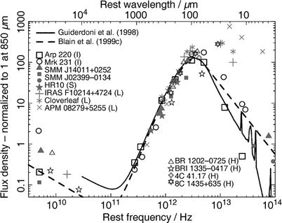
Fig. 9.30
Spectral energy distribution of some dusty
galaxies with known redshift z (symbols), together with two model
spectra (curves). The
spectral distributions for all sources are normalized to unity at
λ = 850 μm. Four types of
galaxies are distinguished: (I) IRAS galaxies at low z; (S) luminous sub-mm galaxies; (L)
distant sources that are magnified by the gravitational lens effect
and multiply imaged; (H) AGNs. Only a few sources among the lens
systems (presumably due to differential magnification) and the AGNs
deviate significantly from the model spectra. Source: A. Blain
et al. 1999, Submillimeter-selected galaxies,
astro-ph/9908111, Fig. 3. Reproduced by permission of the
author
FIR emission from hot dust is one of the best
indicators of star formation. However, observations in this
waveband are only possible from space, such as was done with the
IRAS and ISO satellites, and more recently with Spitzer and
Herschel. Depending on the dust temperature, dust emission has its
maximum at about 100 μm, which is not observable from the ground.
At longer wavelengths there are spectral windows longwards of
λ ∼ 250 μm where
observations through the Earth’s atmosphere are possible, for
instance at 450 and 850 μm in the sub-millimeter waveband. However,
the observing conditions at these wavelengths are extremely
dependent on the amount of water vapor in the atmosphere, so that
the observing sites must by dry and at high elevations. In the
sub-millimeter (sub-mm) range, the long wavelength domain of
thermal dust radiation can be observed, which is illustrated in
Fig. 9.30.

Fig. 9.31
A sub-millimeter image of the COSMOS field,
taken with the SPIRE instrument on Herschel. The image is about
2 degrees on the side and is a color composite of three bands with
wavelength 250, 350 and 500 μm. For six galaxies in the field, the
zooms show an optical images, with the cosmic look-back time
indicated as obtained by spectroscopy with the W.M. Keck
telescopes. Credit: COSMOS field: ESA/Herschel/SPIRE/HerMES Key
Programme; Hubble images: NASA, ESA; Keck Spectra: Caltech/W. M.
Keck Observatory
Developments. Since about 1998 sub-mm
astronomy has experienced an enormous boom, with two instruments
having been put into operation: the Sub-millimeter Common User
Bolometer Array (SCUBA), operating at 450 and 850 μm, with a
field-of-view of 5 arcmin2, and the Max-Planck
Millimeter Bolometer (MAMBO), operating at 1200 μm. Both are
bolometer arrays which initially had 37 bolometers each, but which
later were upgraded to a considerably larger number of bolometers.
With the opening of the 12-m APEX (Atacama Pathfinder Experiment)
telescope (see Fig. 1.28) in Chile, equipped with
powerful instrumentation, a further big step in sub-mm astronomy
was achieved. In addition, the Herschel satellite
(Fig. 1.33), operating at wavelength
between 55 and 670 μm, allowed imaging of large sky areas at these
wavelengths, due to a much lower noise level than can be achieved
from the ground, though with considerably worse spatial resolution
due to the smaller aperture compared to ground-based sub-mm
telescopes. Figure 9.31 shows a Herschel image of the COSMOS
field.
Apart from single-dish observatories,
interferometers operating at these wavelengths yield substantially
higher angular resolution, for example the very successful IRAM
Plateau de Bure interferometer in the French Alps consisting of six
15-m antennas. The Atacama Large Millimeter Array (ALMA; see
Fig. 1.29) with its 54 12-m and 12 7-m
antennas, inaugurated in 2013, marks a huge leap in terms of
resolution and sensitivity in this waveband regime.

Fig. 9.32
Predicted flux from dusty galaxies as a
function of redshift. The bolometric luminosity of these galaxies
is kept constant. The solid
red and the blue dashed
curves show the flux at λ = 850 μm and λ = 175 μm, respectively. On the right, the index β of the dust emissivity is varied, and
the temperature of the dust T d = 38 K is kept fixed.
On the left, β = 1. 5 is fixed and the temperature
is varied. It is remarkable how flat these curves are over a very
wide range in redshift, in particular at 850 μm; this is due to the
very strong negative K-correction which derives from the spectral
behavior of thermal dust emission, shown in Fig. 9.30. Whereas for these
model calculations an Einstein–de Sitter model was assumed, the
behavior is very similar also in Λ-dominated universes. Source:
A. Blain et al. 1999, Submillimeter-selected galaxies,
astro-ph/9908111, Fig. 1. Reproduced by permission of the
author
The negative
K-correction of sub-mm sources. The emission of dust at
these wavelengths is described by a Rayleigh–Jeans spectrum,
modified by an emissivity function that depends on the dust
properties (chemical composition, distribution of dust grain
sizes); typically, one finds
 This steep spectrum for frequencies below the peak of the thermal
dust emission at λ ∼ 100 μm
implies a very strong negative K-correction (see Sect. 5.6.1) for wavelengths in the
sub-mm domain: at a fixed observed wavelength, the rest-frame
wavelength becomes increasingly smaller for sources at higher
redshift, and there the emissivity is larger. As Fig. 9.32 demonstrates, this
spectral behavior causes the effect that the flux in the sub-mm
range does not necessarily decrease with redshift. For z ≲ 1, the 1∕D 2-dependence of the flux
dominates, so that up to z ∼ 1 sources at fixed luminosity get
fainter with increasing z.
However, between z ∼ 1 and
z ∼ z flat the sub-mm flux as a
function of redshift remains nearly constant or even increases with
z, where z flat depends on the dust
temperature T d
and the observed wavelength; for T d ∼ 40 K and λ ∼ 850 μm one finds z flat ∼ 8. We therefore
have the quite amazing situation that sources appear brighter when
they are at larger distances. This is caused by the very negative
K-correction which more than compensates for the 1∕D 2-decrease of the flux.
Only for z > z
flat does the flux begin to rapidly decrease with
redshift, since then, due to redshift, the corresponding restframe
frequency is shifted to the far side of the maximum of the dust
spectrum (see Fig. 9.30). Hence, a sample of galaxies that is
flux-limited in the sub-mm domain should have a very broad
z-distribution. The dust
temperature is about T
d ∼ 20 K for low-redshift spirals, and T d ∼ 40 K is a typical
value for galaxies at higher redshift featuring active star
formation. The higher T
d, the smaller the sub-mm flux at fixed bolometric
luminosity.
This steep spectrum for frequencies below the peak of the thermal
dust emission at λ ∼ 100 μm
implies a very strong negative K-correction (see Sect. 5.6.1) for wavelengths in the
sub-mm domain: at a fixed observed wavelength, the rest-frame
wavelength becomes increasingly smaller for sources at higher
redshift, and there the emissivity is larger. As Fig. 9.32 demonstrates, this
spectral behavior causes the effect that the flux in the sub-mm
range does not necessarily decrease with redshift. For z ≲ 1, the 1∕D 2-dependence of the flux
dominates, so that up to z ∼ 1 sources at fixed luminosity get
fainter with increasing z.
However, between z ∼ 1 and
z ∼ z flat the sub-mm flux as a
function of redshift remains nearly constant or even increases with
z, where z flat depends on the dust
temperature T d
and the observed wavelength; for T d ∼ 40 K and λ ∼ 850 μm one finds z flat ∼ 8. We therefore
have the quite amazing situation that sources appear brighter when
they are at larger distances. This is caused by the very negative
K-correction which more than compensates for the 1∕D 2-decrease of the flux.
Only for z > z
flat does the flux begin to rapidly decrease with
redshift, since then, due to redshift, the corresponding restframe
frequency is shifted to the far side of the maximum of the dust
spectrum (see Fig. 9.30). Hence, a sample of galaxies that is
flux-limited in the sub-mm domain should have a very broad
z-distribution. The dust
temperature is about T
d ∼ 20 K for low-redshift spirals, and T d ∼ 40 K is a typical
value for galaxies at higher redshift featuring active star
formation. The higher T
d, the smaller the sub-mm flux at fixed bolometric
luminosity.
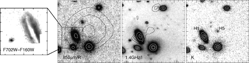
Fig. 9.33
The sub-mm galaxy SMM J09429+4658. The
three images on the right
have a side length of 30″ each, centered on the center of the error
box of the 850 μm observation. The smaller image on the left is the difference of two
HST images in red and infrared filters, showing the dust disk in
the spiral galaxy H1. The second
image from the left displays an R-band image, superposed
with the contours of the SCUBA 850 μm emission. The second image from the right is an
I-band image, superposed with the contours of radio emission at
1. 4 GHz, and the right-most
panel shows a K-band image. The radio contours show emission
from the galaxy H1 (z = 0. 33), but also weaker emission
right at the center of the sub-mm map. In the K-band, a NIR source
(H5) is found exactly at this position. It remains unclear which of
these two sources is the sub-mm source, but the ratio of sub-mm to
1. 4 GHz emission would be atypical if H1 is identified with the
sub-mm source. Source: A. Blain et al. 1999, Submillimeter-selected galaxies,
astro-ph/9908111, Fig. 4. Reproduced by permission of the
author
Counts of sub-mm sources at high Galactic
latitudes have yielded a far higher number density than was
predicted by early galaxy evolution models. For the density of
sources as a function of limiting flux S, at wavelength λ = 850 μm, one obtains

(9.1)
The identification
of sub-mm sources. At first, the optical identification of
these sources turned out to be extremely difficult: due to the
relatively low angular resolution of single-dish sub-millimeter
telescopes (for example, MAMBO has a beam with FWHM of ∼ 11″ at
λ = 1. 2 mm), the positions
of sources can only be determined with an accuracy of several
acrseconds.5
Typically, several faint galaxies can be identified on deep optical
images within an error circle of this radius. Furthermore,
Fig. 9.32
suggests that these sources have a relatively high redshift, thus
they should be very faint in the optical. An additional problem is
reddening and extinction by the same dust that is the source of the
sub-mm emission.
The identification of sub-mm sources was finally
accomplished by means of their radio emission, since a majority of
the sources selected at sub-mm wavelengths can be identified in
very deep radio observations at 1. 4 GHz. Since the radio sky is
far less crowded than the optical one, and since the VLA achieves
an angular resolution of ∼ 1″ at λ = 20 cm, the optical identification
of the corresponding radio source becomes relatively easy. One
example of this identification process is shown in
Fig. 9.33.
With the accurate radio position of a sub-mm source, the optical
identification can then be performed. In most cases, they are very
faint optical sources indeed, so that spectroscopic analysis is
difficult and very time-consuming. Another method for estimating
the redshift results from the spectral energy distribution shown in
Fig. 9.30.
Since this spectrum seems to be nearly universal, i.e., not varying
much among different sources, some kind of photometric redshift can
be estimated from the ratio of the fluxes at 1.4 GHz and 850 μm,
yielding reasonable estimates in many cases.
Redshift
distribution of SMGs. The median redshift of sources with
850 μm flux larger than 5 mJy and 1. 4 GHz flux above 30 μJy is
about 2.2. However, at these sensitivities about half the sub-mm
sources are unidentified in the radio, and hence their redshift
distribution could be different from those with radio counterparts.
In some of the sources with radio identification, an AGN component,
which contributes to the dust heating, was identified, but in
general newly born stars seem to be the prime source of the
energetic photons which heat the dust. The optical morphology and
the number density of the sub-mm sources suggest that we are
witnessing the formation of massive elliptical galaxies in these
sub-mm sources.
The great capabilities of interferometric
observations enables a different method for identification and
redshift determination of SMGs. The high angular resolution of the
Plateau de Bure and, in particular, ALMA interferometers can
pinpoint a sub-mm source very accurately, allowing the
identification with optical or infrared sources. In addition, the
large bandwidth of the ALMA receivers can take spectra of these
sources over an appreciable range of wavelengths, and thus identify
emission lines of molecules, predominantly those of the CO and
water molecules, or fine-structure lines of atoms (specifically,
ionized and neutral carbon), therefore removing the need for
obtaining optical spectra of these optically faint sources. The
potential of this method was recently established: even by
observing with an incomplete array of telescopes, ALMA detected
emission lines in 23 out of 26 sources selected by the South Pole
Telescope (SPT; see Fig. 1.31) at 1. 4 mm wavelength.
Once the precise locations of the sub-mm sources
are determined with interferometric observations, they can be
identified on deep optical images, and their redshifts be
determined from optical spectroscopy. Hence, much of the potential
bias in the redshift distribution of these sources, which are
caused by the fact that only about half of the SMGs have a radio
identification, are removed.6 Indeed, if one compares the redshift
distributions of both samples, shown in Fig. 9.34, one sees that they
are significantly different. Using radio-identification as an
intermediate step, and neglecting those SMGs for which no radio
source could be identified, biases the redshift distribution of
dusty star-forming galaxies low. The population extends over a
significantly larger redshift range than concluded previously—in
accord with expectations from the large negative K-correction. In
addition, the redshifts of SMGs can be determined with the PdB and
ALMA interferometers directly, using molecular line spectroscopy,
without the need for optical spectroscopy. In particular the large
bandwidth of the ALMA receiver allows one to cover a broad range of
wavelengths, and thus of redshifts for which molecular lines can be
detected and identified.

Fig. 9.34
The grey
line shows the cumulative redshift distribution of dusty
star-forming galaxies selected from the SPT survey, as determined
by molecular line spectroscopy with ALMA; the distribution has a
median redshift of z
med ∼ 3. 5. The blue
curve is the redshift distribution of SMGs that were
identified with radio sources and subsequently their redshift was
determined by optical spectroscopy, yielding z med ∼ 2. 2. The
orange curve is the
redshift distribution of SMGs identified at mm-wavelengths, with
redshifts determined mainly through photometric fitting. Source:
J.D. Vieira et al. 2013, Dusty starburst galaxies in the early Universe
as revealed by gravitational lensing, Nature 495, 344,
Fig. 3. Reprinted by permission of Macmillan Publishers Ltd:
Nature, ©2013
Halo masses of
sub-mm galaxies. As we discussed in Sect. 8.1.2, one can estimate the mass of
the dark matter halo in which objects reside, by comparing their
clustering properties with those of dark matter halos, as obtained
from cosmological simulations. Sub-mm galaxies identified in a
survey conducted by APEX (see the left panel of Fig. 9.35) allowed an estimate
of the clustering length r
0 (defined such that the two-point correlation function
is unity at separation r
0) of these sources, yielding r 0 ≈ (7. 5 ± 2)h −1 Mpc. In the right panel
of Fig. 9.35,
this measurement of r
0 is related to that of other source populations. The
clustering length of sub-mm sources is very similar to that of QSOs
at the same redshift, and considerably larger than that for
Lyman-break galaxies. Comparing this to the clustering length of
dark matter halos with different masses, shown as dotted curves in
Fig. 9.35, we
conclude that SMGs live in relatively massive halos of several
times 1012 M
⊙ at z ∼ 2. This
results was recently confirmed by detecting a weak lensing signal
around a sample of ∼ 600 relatively bright SMGs, which yields a
characteristic halo mass of these galaxies of ∼ 1013
M ⊙. This mass
is comparable to that of current epoch massive elliptical galaxies,
and suggests the interpretation that high-redshift SMGs evolve into
present-day ellipticals. A large fraction of their stellar
population is formed in the epoch at which the galaxy is seen as a
SMG; by the end of this period, most of the gas in the galaxy is
used up (or some fraction of it may be expelled), and in the
remaining evolution little or no star formation occurs.
Additional support for this idea is provided by
the fact that the sub-mm galaxies are typically brighter and redder
than (restframe) UV-selected galaxies at redshifts z ∼ 2. 5. This indicates that the
stellar masses in sub-mm galaxies are higher than those of
LBGs.
A joint investigation of z ∼ 2 sub-mm galaxies at X-ray, optical
and MIR wavelengths yields that these sources are not only forming
stars at a high rate, but that they already contain a substantial
stellar population with M ∼ 1011 M ⊙, roughly an order of
magnitude more massive than LBGs at similar redshifts. The large
AGN fraction among sub-mm galaxies indicates that the growth of the
stellar population is accompanied by accretion and thus the growth
of supermassive black holes in these objects. Nevertheless, the
relatively faint X-ray emission from these galaxies suggests that
either their SMBHs have a mass well below the local relation
between M • and
stellar properties of (spheroidal) galaxies, or that they accrete
at well below the Eddington rate. Furthermore, the typical ratio of
X-ray to sub-mm luminosity of these sources is about one order of
magnitude smaller than in typical AGNs, which seems to imply that
the total luminosity of these sources is dominated by the
star-formation activity, rather than by accretion power. This
conclusion is supported by the fact that the optical counterparts
of SMGs show strong signs of merging and interactions, together
with their larger size compared to optically-selected galaxies at
the same redshifts. This latter point shows that the emission comes
from an extended region, as expected from star formation in
mergers, rather than AGN activity.

Fig. 9.35
Left
panel: Sub-millimeter sources in the Extended Chandra Deep
Field South (ECDFS). The image shows highly significant detections
of sub-mm sources at 870 μm, as observed with the 12-m APEX
telescope, superimposed on a Spitzer mid-IR image of the same sky
region. On the 0. 35 deg2 of the ECDFS, 126 sub-mm
sources were detected with a significance higher than
3. 7σ. Right panel: Based on a clustering
analysis of the sub-mm sources shown on the left, the clustering length
r 0 of the
sources was determined. The figure shows the clustering length as a
function of redshift, for different types of sources: QSOs over a
broad range of redshifts, local ellipticals and luminous red
galaxies, local blue galaxies and star-forming galaxies at
intermediate redshift, as selected by Spitzer at 24 μm wavelength,
high-redshift Lyman-break galaxies, and galaxy clusters. The
dotted curves indicate the
clustering length of dark matter halos as a function of redshift,
for different halo masses as indicated. Credit: Left: ESO, APEX (MPIfR/ESO/OSO), A.
Weiss et al., NASA Spitzer Science Center. Right: R.C. Hickox et
al. 2012, The LABOCA survey
of the Extended Chandra Deep Field-South: clustering of
submillimetre galaxies, MNRAS 421, 284, p. 291, Fig. 6b.
Reproduced by permission of Oxford University Press on behalf of
the Royal Astronomical Society

Fig. 9.36
The sub-millimeter galaxy HXMM01, detected
by Herschel in the framework of the HerMES survey. In blue, a K-band image shows the presence
of four main sources in this field; the two big ones are galaxies
at z = 0. 66 (left) and z = 0. 50 (right). The two smaller ones, separated
by ∼ 3″, are at the same redshift of z = 2. 31. In red, a sub-millimeter maps is shown,
whereas green displays
molecular emission. The two yellow
spots show the regions where near-IR, sub-mm and molecular
emission are spatially coincident; from those regions, the bulk of
the flux seen by Herschel is emitted. The image has a size of about
10″ on a side. Credit: ESA/NASA/JPL-Caltech/UC
Irvine/STScI/Keck/NRAO/SAO
Merging
SMGs. The Herschel satellite found a strong sub-mm source,
whose subsequent reobservations with different telescopes revealed
this to be a merger of two SMGs. This source, called HXMM01, is
shown in Fig. 9.36. In the near-IR, the image shows four main
sources, of which the two brightest ones are galaxies at
intermediate redshifts. The two fainter ones are galaxies at
z = 2. 31. Those coincide
with strong sub-mm sources, as seen by the interferometric images
at 880 μm, as well as through their strong molecular line emission.
This pair of sources has a separation of 19 kpc, and is most likely
undergoing a merger. The two foreground galaxies will cause a
moderate lensing magnification of the SMGs, with an estimated
μ ∼ 1. 6. Thus, even after
magnification correction, this source belongs to the brightest
SMGs, with a corrected flux of ∼ 20 mJy at λ = 850 μm. This source is extreme in
several properties: Its dust temperature is estimated to be
T ≈ 55 K, which is larger
than that of most starburst galaxies. The estimated bolometric
infrared luminosity is L ∼ 2 × 10¹³ L ⊙, with a corresponding
star-formation rate of  . At this
rate, the molecular gas of ∼ 2. 3 × 10¹¹ M ⊙ will be turned into
stars on a timescale of only 70 Myr. The brevity of this time
interval implies that objects similar to HXMM01 should be rare. The
molecular gas mass in this object is comparable with the stellar
mass already present, i.e., the gas-mass fraction in this object is
about 50 %. At the end of its merging process and star-formation
episode, the resulting galaxy will have a stellar mass
of ∼ 1011 M
⊙, i.e., the stellar mass of a massive elliptical
galaxy.
. At this
rate, the molecular gas of ∼ 2. 3 × 10¹¹ M ⊙ will be turned into
stars on a timescale of only 70 Myr. The brevity of this time
interval implies that objects similar to HXMM01 should be rare. The
molecular gas mass in this object is comparable with the stellar
mass already present, i.e., the gas-mass fraction in this object is
about 50 %. At the end of its merging process and star-formation
episode, the resulting galaxy will have a stellar mass
of ∼ 1011 M
⊙, i.e., the stellar mass of a massive elliptical
galaxy.Although HXMM01 is not the only pair of merging
SMGs yet discovered, it is brighter than the other ones by a factor
of ∼ 2 (magnification corrected); correspondingly, its
star-formation rate is also about twice that of the other merging
systems. There are indications that the far-IR luminosity, and thus
the star-formation rate, at fixed molecular mass (as measured by
the luminosity in molecular CO lines), is higher by about a factor
of three compared to galaxies that are not observed to be merging.
This then is a direct hint at the possibility that merging triggers
star-formation events, or bursts of star-formation.
In fact, there are several observations which
suggest that the very large star-forming rates of many of the most
luminous SMGs are due to merging events. Arguably the most direct
one comes from interferometric observations of the molecular gas in
SMGs, which shows that most of them have morphological and
kinematical properties that identify them as merging systems.
Hence, in accordance with the high merger rate of local ULIRGs, the
extreme SMGs may also be triggered by merger events.
If dusty galaxies are at very high redshifts
z ≳ 5, the peak of their
spectral energy distribution shown in Fig. 9.30 is observed at
wavelengths longward of 500 μm. Hence, for such sources the flux
density is expected to increase with wavelength for λ ≲ 500 μm. The SPIRE instrument on the
Herschel Space Observatory observed at 250, 350 and 500 μm, and
blank survey fields at these frequencies can thus be used to search
for very high-redshift sub-millimeter galaxies.
One such object found by this selection method is
shown in Fig. 9.37. The galaxy HFLS3 is an extreme starburst
at z = 6. 34, with an
estimated star-formation rate of ∼ 3000 M ⊙∕yr, some factor of 20
larger than the local starburst Arp 220 (see Fig. 1.15). With an estimated gas mass
of ∼ 1011 M
⊙, this object would transform all its gas mass into
stars on a time-scale of only ∼ 30 Myr, assuming a constant
star-formation rate. Spatially resolved molecular spectroscopy
shows a velocity profile of this galaxy, which can be used to
estimate a dynamical mass of ∼ 2. 7 × 10¹¹ M ⊙, yielding a gas-mass
fraction of ∼ 40 %, similar to what is found in typical
z ∼ 2 sub-millimeter
galaxies.
Magnification bias
of sub-millimeter sources. We mentioned before that some of
the apparently most luminous sources of any kind have a large
probability of being gravitationally lensed. The reason for this
can be seen as follows: If we consider a population of sources,
then their distribution in luminosity is most frequently described
by a Schechter-like function. That means that for low luminosities,
the luminosity function behaves as a power law in L, whereas for L > L ∗, where L ∗ characterizes the break
in the luminosity function, the density of sources decreases
exponentially with L. In
particular that means that there are essentially no sources with
luminosity L ≳ 5L
∗.
The probability that any given high-redshift
source is gravitationally lensed and significantly magnified is
small, of order 10−4. Thus, if one picks random sources,
the fraction of lensed ones among them will be similarly small.
However, we can not pick random sources, but only sources above the
flux limit of our observations. The situation in flux-limited
samples can be quite different, since the magnification by lensing
affects the mix of sources which are above the flux threshold. The
probability that a source undergoes a magnification larger than
μ can be shown to behave
like μ −2,
provided the source is sufficiently small. Hence, large
magnifications are correspondingly rare. But the probability for
large magnifications decreases as a power law in μ—compared to the exponential decrease
in the luminosity of sources for L > L ∗. There will be a point
where the (low-amplitude) power law overtakes the exponential, or
in other words, where a source above a given flux threshold is more
likely to be highly magnified, than having a very high intrinsic
luminosity. An example of this effect are the bright z ∼ 3 Lyman-break galaxies shown in
Figs. 9.17
and 9.18,
whose inferred luminosity is much larger than the L ∗ of this population of
galaxies.

Fig. 9.37
The galaxy HFLS3 at z = 6. 34, found by a color selection
in the sub-millimeter regime. The big image shows a part of the
HerMES blank field survey, with cut-outs at different wavelengths
shown as small panels on the right, as well as an optical image and
one combining near-IR and millimeter imaging.
Credit: ESA/Herschel/HerMES/ IRAM/GTC/W.M. Keck
Observatory
This is illustrated in Fig. 9.38, where the upper end
of the 500 μm source counts are shown, together with a model
decomposition of the counts into lensed and unlensed SMGs, nearby
spiral galaxies and radio AGNs. As we just argued, for relatively
low fluxes, the fraction of lensed sources is increasingly small.
However, due to the steep decline of the unlensed counts, beyond a
certain flux level they start to dominate the counts of SMGs. From
that figure, one therefore expects that a SMG with S ≳ 60 mJy at 500 μm has a fairly high
probability of being lensed, whereas a SMG with S ≳ 100 mJy almost certainly is a
lensed source.
Hence, selecting sources with S ≳ 100 mJy, and cleaning the source
catalog for nearby spirals (they are bright and big in the optical,
and can thus easily be identified), one expects to obtain a clean
lensed sample. Indeed, all five candidates selected from the survey
data on which Fig. 9.38 is based, are most likely lensed, with the
putative lens being identified on optical and NIR images.
Furthermore, interferometric observations have confirmed the
lensing nature of several of the candidates, by finding multiple
images.
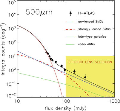
Fig. 9.38
The dominance of gravitationally-lensed
magnified sub-mm galaxies at the bright end. The dots show the upper end of the 500 μm
source counts of SMGs, obtained from the Herschel ATLAS survey. The
red curve shows a model of
the unlensed source counts, which has the shape of a
Schechter-function, and drops off exponentially for large
S. The red dashed curve shows the
corresponding counts of lensed and magnified sources, whereas the
blue curve is the
contribution from low-redshift spiral galaxies. The lensed SMGs
overtake the unlensed ones for fluxes ≳ 60 mJy. Source:
M. Negrello et al. 2010, The Detection of a Population of
Submillimeter-Bright, Strongly-Lensed Galaxies,
arXiv:1011.1255, Fig. 1. Reproduced by permission of the
author
Using ALMA imaging of sources from the South Pole
Telescope survey, selected at 1.4 and 2 mm to have the spectral
index at these wavelengths corresponding to dust, and cleaning the
sample for nearby objects (e.g., excluding sources detected by IRAS
or in low-frequency radio catalogs), a large fraction of these
sources turn out to be gravitationally lensed. In Fig. 9.39, ten of these are
shown, where not only the multiple images of the sources (which are
all at high redshift) are shown, but also a near-IR image of the
field which clearly shows the lensing galaxy. Hence, selecting
bright sources in the (sub)-millimeter regime yields a very high
success rate of finding gravitational lens systems. All these lens
systems would be missed in optical surveys, due to the faintness of
the SMGs at optical and NIR wavelengths.
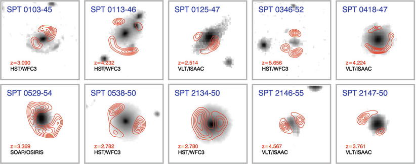
Fig. 9.39
Near-infrared (greyscale) and ALMA 870 μm
images of ten high flux millimeter-selected sources from the South
Pole Telescope survey. The redshifts of the SMGs are indicated in
the lower left corner of
each panel. All ten sources are obviously gravitationally lensed by
a foreground galaxy. Source: J.D. Vieira et al. 2013,
Dusty starburst galaxies in the
early Universe as revealed by gravitational lensing,
arXiv:1303.2723, Fig. 1. Reproduced by permission of the
author
9.3.4 Damped Lyman-alpha systems
In our discussion of QSO absorption lines in
Sect. 5.7, we mentioned that the
Lyα lines are broadly
classed into three categories: the Lyα forest, Lyman-limit systems, and
damped Lyα systems, which
are separated by a column density of N
HI ∼ 1017 cm−2 and N HI ∼ 2 ×
1020 cm−2, respectively. The origin of the
Lyα forest, as discussed in
some detail in Sect. 8.5, is diffuse, highly ionized gas
with small density contrast. In comparison, the large column
density of damped Lyα
systems (DLAs) strongly suggests that hydrogen is mostly neutral in
these systems. The reason for this is self-shielding : for column
densities of N
HI ≳ 2 × 1020 cm−2 the background
of ionizing photons is unable to penetrate deeply into the
corresponding hydrogen ‘cloud’, so that only its surface is highly
ionized. Interestingly enough, this column density is about the
same as that observed in 21 cm hydrogen emission at the optical
radius of nearby spiral galaxies.
DLAs can be observed at all redshifts
z ≲ 5. For z > 5 the Lyα forest becomes so dense that these
damped absorption lines are very difficult to identify. For
z ≲ 1. 6 the Lyα transition cannot be observed from
the ground; since the apertures of optical/UV telescopes in space
are considerably smaller than those on the ground, low-redshift
DLAs are substantially more complicated to observe than those at
higher z.
The neutral
hydrogen mass contained in DLAs. The column density
distribution of Lyα forest
lines is a power law, given by (8.30). The relatively flat slope of
β ∼ 1. 6 indicates that
most of the neutral hydrogen is contained in systems of high column
density. This can be seen as follows: the total column density of
neutral hydrogen above some minimum column density N min is
 and is, for β < 2,
dominated by the highest column density systems. In fact, unless
the distribution of column densities steepens for very high
N HI, the
integral diverges. From the extended statistics now available for
DLAs, it is known that dN∕dN HI attains a break at
column densities above N
HI ≳ 1021 cm−2, rendering the
above integral finite. Nevertheless, this consideration implies
that most of the neutral hydrogen in the Universe visible in QSO
absorption lines is contained in DLAs. From the observed
distribution of DLAs as a function of column density and redshift,
the density parameter Ω
HI in neutral hydrogen as a function of redshift can be
inferred. Apparently, Ω
HI ∼ 10−3 over the whole redshift interval
0 < z < 5, with
perhaps a small redshift dependence. Compared to the current
density of stars, this neutral hydrogen density is smaller only by
a factor ∼ 3. Therefore, the hydrogen contained in DLAs is an
important reservoir for star formation, and DLAs may represent
condensations of gas that turn into ‘normal’ galaxies once
star-formation sets in. Since DLAs have low metallicities,
typically 1/10 of the Solar abundance, it is quite plausible that
they have not yet experienced much star formation.
and is, for β < 2,
dominated by the highest column density systems. In fact, unless
the distribution of column densities steepens for very high
N HI, the
integral diverges. From the extended statistics now available for
DLAs, it is known that dN∕dN HI attains a break at
column densities above N
HI ≳ 1021 cm−2, rendering the
above integral finite. Nevertheless, this consideration implies
that most of the neutral hydrogen in the Universe visible in QSO
absorption lines is contained in DLAs. From the observed
distribution of DLAs as a function of column density and redshift,
the density parameter Ω
HI in neutral hydrogen as a function of redshift can be
inferred. Apparently, Ω
HI ∼ 10−3 over the whole redshift interval
0 < z < 5, with
perhaps a small redshift dependence. Compared to the current
density of stars, this neutral hydrogen density is smaller only by
a factor ∼ 3. Therefore, the hydrogen contained in DLAs is an
important reservoir for star formation, and DLAs may represent
condensations of gas that turn into ‘normal’ galaxies once
star-formation sets in. Since DLAs have low metallicities,
typically 1/10 of the Solar abundance, it is quite plausible that
they have not yet experienced much star formation.
(9.2)
The nature of
DLAs. This interpretation is supported by the kinematical
properties of DLAs. Whereas the fact that the Lyα line is damped implies that its
observed shape is essentially independent of the Doppler velocity
of the gas, velocity information can nevertheless be obtained from
metal lines. Every DLA is associated with metal absorption line
systems, covering low- and high-ionization species (such as
Siii and Civ, respectively) which can be
observed by choosing the appropriate wavelength coverage of the
spectrum. The profiles of these metal lines are usually split up
into several components. Interpreted as ionized ‘clouds’, the
velocity range Δ v thus
obtained can be used as an indicator of the characteristic
velocities of the DLA. The values of Δ v cover a wide range, with a median
of ∼ 90 km∕s for the low-ionization lines and ∼ 190 km∕s for the
high-ionization transitions. The observed distribution is largely
compatible with the interpretation that DLAs are rotating disks
with a characteristic rotational velocity of v c ∼ 200 km∕s, once random
orientations and impact parameters of the line-of-sight to the QSO
are taken into account.
Search for
emission from DLAs. If this interpretation is correct, then
we might expect that the DLAs can also be observed as galaxies in
emission. This, however, is exceedingly difficult for the
high-redshift DLAs. Noting that they are discovered as absorption
lines in the spectrum of QSOs, we face the difficulty of imaging a
high-redshift galaxy very close to the line-of-sight to a bright
QSO (to quote characteristic numbers, the typical QSO used for
absorption-line spectroscopy has B ∼ 18, whereas an L ∗-galaxy at z ∼ 3 has B ∼ 24. 5). Due to the size of the
point-spread function this is nearly hopeless from the ground. But
even with the resolution of HST, it is a difficult undertaking.
Another possibility is to look for the Lyα emission line at the absorption
redshift, located right in the wavelength range where the DLA fully
blocks the QSO light. However, as we discussed for LBGs above, not
all galaxies show Lyα in
emission, and it is not too surprising that these searches have
largely failed. Only very few DLA have been detected in emission,
with some of them seen only through the Lyα emission line at the trough of the
damped absorption line, but with no observable continuum radiation.
This latter fact indicates that the blue light from DLAs is
considerably fainter than that from a typical LBG at z ∼ 3, consistent with the
interpretation that DLAs are not strong star-forming objects. But
at least one DLA is observed to be considerably brighter and seems
to share some characteristics of LBGs, including a high
star-formation rate. In addition, a couple of DLAs have been
detected by [Oiii]
emission lines. Overall, then, the nature of high-redshift DLAs is
still unclear, due to the small number of direct
identifications.
For DLAs at low redshifts the observational
situation is different, in that a fair fraction of them have
counterparts seen in emission. Whereas the interpretation of the
data is still not unambiguous, it seems that the low-redshift
population of DLAs may be composed of normal galaxies.
The spatial abundance of DLAs is largely unknown.
The observed frequency of DLAs in QSO spectra is the product of the
spatial abundance and the absorption cross section of the
absorbers. This product can be compared with the corresponding
quantity of local galaxies: the detailed mapping of nearby galaxies
in the 21 cm line shows that their abundance and gaseous cross
section are compatible with the frequency of DLAs for z ≲ 1. 5, and falls short by a
factor ∼ 2 for the higher-redshifts DLAs.
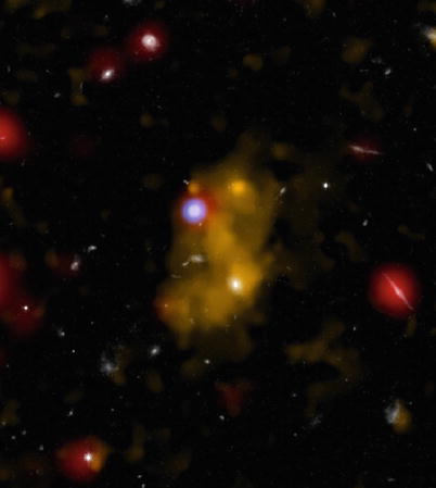
Fig. 9.40
Composite image of a Lyα blob at z = 3. 09. The yellow color shows the Lyα emission, obtained by a narrow-band
filter exposure. Inside the blob a galaxy is located, as seen in an
optical (white) and
infrared (8 μm, red)
broadband image. X-ray emission (shown in blue) indicates that the Lyα emission is powered by an AGN. This
image has a size of 38″. Credit: X-ray (NASA/CXC/Durham
Univ./D.Alexander et al.); Optical (NASA/ESA/STScI/IoA/S.Chapman et
al.); Lyman-alpha Optical (NAOJ/Subaru/Tohoku Univ./T.Hayashino et
al.); Infrared (NASA/JPL-Caltech/Durham Univ./J.Geach et al.)
9.3.5 Lyman-alpha blobs
The search for high-redshift galaxies with
narrow-band imaging, where the filter is centered on the redshifted
Lyα emission line, has
revealed a class of objects which are termed ‘Lyman-α blobs’. These are luminous and very
extended sources of Lyα
emission; their characteristic flux in the Lyα line is ∼ 1044 erg∕s, and
their typical size is ∼ 30 to ∼ 100 kpc. Some of these sources show
no detectable continuum emission in any broad-band optical filter.
Hence, these sources seem to form a distinct class from the
Lyman-alpha emitters discussed previously.
The nature of these high-redshifts objects
remained unknown for a long time. Suggested explanations were
wide-ranging, including a hidden QSO, strong star formation and
associated superwinds, as well as ‘cold accretion’, where gas is
accreted onto a dark matter halo and hydrogen is collisionally
excited in the gas of temperature ∼ 104 K, yielding the
observed Lyα emission. It
even seems plausible that the Lyman-α blobs encompass a range of different
phenomena, and that all three modes of powering the line emission
indeed occur. As a common feature, most of the Lyman-α blobs are associated with luminous
galaxies, and are associated with strong infrared emission.
Chandra observations of 29 Lyα blobs detected five on them in
X-rays; one of them is shown in Fig. 9.40. The X-ray sources
are AGNs with L
X ∼ 1044 erg∕s and rather large obscuration.
Furthermore, these sources emit infrared light from warm dust. The
energy output of the AGN is sufficiently large to power the
Lyα emission through
photoionization. Hence, the AGN hypothesis has been verified for at
least some of the sources.
Two of these Lyα blobs were discovered by narrow-band
imaging of the aforementioned proto-cluster of LBGs at z = 3. 09. Both of them are sub-mm
sources and therefore star-forming objects; the more powerful one
has a sub-mm flux suggesting a star-formation rate
of ∼ 1000M ⊙∕yr.
Spatially resolved spectroscopy extending over the full ∼ 100 kpc
size of one of the Lyα
blobs shows that across the whole region there is an absorption
line centered on the Lyα
emission line. The optical depth of the absorption line suggests an
Hi column density
of ∼ 1019 cm−2, and its centroid is
blueshifted relative to the underlying emission line by ∼ 250 km∕s.
The spatial extent of the blueshifted absorption shows that the
outflowing material is a global phenomenon in this object—a true
superwind, most likely driven by energetic star formation and
subsequent supernova explosions in these objects. Therefore, it
appears likely that Lyα
blobs are intimately connected to massive star-formation
activity.
9.4 Properties of galaxies at high redshift
9.4.1 Demography of high-redshift galaxies
Being able to detect galaxies at high redshifts,
we may first consider their abundance and investigate how their
luminosity distribution compares with that galaxies in the local
Universe. We are interested in a possible evolution of the
luminosity function of galaxies with redshift, as this would
clearly indicate that the galaxy population as a whole changes with
redshift. The source counts from the Hubble Deep Field
(Fig. 9.11)
and its strong deviations from the non-evolution models provide a
clear indication that the galaxy population evolves in redshift.
This point will be considered here in somewhat more detail.
The most convenient way of summarizing the
results is a representation of the estimated luminosity function in
terms of a fit with a Schechter function (3.52). In that, the luminosity
function is characterized by an overall normalization Φ ∗, a characteristic
luminosity L ∗
(or, equivalently, an absolute magnitude M ∗) above which the
abundance decreases exponentially, and a power-law slope
α of the luminosity
function at L ≪ L
∗. An evolution of Φ ∗ with redshift indicates
that the abundance of luminous galaxies evolves. If L ∗ depends on z, one may conclude that the luminosity
of a typical galaxy is different at higher redshifts. Finally, the
faint-end slope α
determines what fraction of the total luminosity of the galaxy
population is emitted by the fainter
galaxies—see (3.58).
The UV-luminosity
function. Since high-redshift galaxies are selected using
quite a variety of methods, as discussed in Sect. 9.1, and since the nature
of the detected galaxies depends on their selection method, one has
to consider different types of luminosity functions. For example,
the Lyman-break method selects galaxies by their rest-frame UV
radiation, so that from these surveys, the UV-luminosity function
of galaxies can be obtained. Since the Lyman-break technique is
applicable over a very wide redshift range, the UV-luminosity
function has been obtained for redshifts between 2 and 7.
As already indicated by the galaxy counts shown
in Fig. 9.11,
the rest-frame UV-luminosity function of galaxies evolves strongly
with redshift. In the redshift interval 2 ≲ z ≲ 4, the characteristic luminosity
L ∗ is about
three magnitudes brighter than that of the local UV-luminosity
function as determined with GALEX. This immediately shows that a
typical galaxy at these redshifts is far more actively forming
stars than local galaxies. Furthermore, the faint-end slope
α is steeper for the
high-redshift galaxies than for local ones. In fact, estimates
yield α ∼ −1. 6, indicating
that much of the UV-luminosity density at high redshifts is emitted
from rather faint galaxies—galaxies which are currently not
observed due to the limited sensitivity of our instruments.
Therefore, the overall abundance of UV-luminous galaxies is
considerably larger in the redshift interval 2 ≲ z ≲ 4 than it is today. Since the
UV-radiation is produced by massive (and thus young) stars, this
implies that the star-formation activity at those redshifts was
much more intense than at the current epoch.
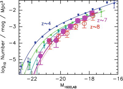
Fig. 9.41
High-redshift rest-frame UV luminosity
functions of galaxies, obtained from data of the Hubble Deep Fields
described in Sect. 9.2. Shown in blue, green and cyan are the luminosity functions at
redshifts z ∼ 4, 5, and 6,
respectively, whereas the magenta and red circles show the estimated
luminosity functions at z ∼ 7 and 8. The curves show a Schechter-function fit to
the data. Source: R.J. Bouwens et al. 2011, Ultraviolet Luminosity Functions from 132
z ∼ 7 and z ∼ 8
Lyman-break Galaxies in the
Ultra-deep HUDF09 and Wide-area Early Release Science WFC3/IR
Observations, ApJ 737, 90, p. 16, Fig. 12. ©AAS. Reproduced
with permission
Going to even higher redshifts, the abundance of
UV-selected galaxies decreases again, as can be seen in
Fig. 9.41.
The evolution is such that the characteristic luminosity decreases
with higher z, and at the
same time the faint-end slope steepens towards an estimated value
of α ∼ −1. 8. Hence, for
these very high redshifts, most of the luminosity in the UV is
emitted from faint sources. Recent attempts to find credible
z ∼ 10 galaxies using the
Lyman-break technique yielded upper limits to the abundance of
these objects, which yields upper limits to the luminosity function
at this redshift. It appears that the decrease with z, visible in Fig. 9.41, accelerates towards
even higher redshift.
In detail, these results are still burdened with
quite some uncertainties, given the difficulties to identify very
high redshift sources. Most of the conclusions are based on
photometric redshifts only, since the spectroscopic verification of
a z ∼ 7 galaxy is extremely
difficult, given that all spectral features blueward of the
Lyα emission line are
invisible due to intergalactic absorption, and that the radiation
redward of the Lyα-line is
redshifted into the near-IR. Hence, some of the sources may be
misidentified and are in fact lower-redshift objects. Furthermore,
since the identification of these very high redshift sources
requires very deep observations, carried out only in a small number
of fields, one must be aware of sampling variance—the fact that the
distribution in a single small field may not be representative of
the overall distribution. However, the general trends just
discussed are established by now, providing a clear view of the
evolution of the galaxy population with cosmic time.
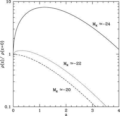
Fig. 9.42
The comoving number density of galaxies
with fixed rest-frame K-band luminosity, normalized by their
current space density, as a function of redshift. The very
different redshift dependence of high- and low-luminosity galaxies,
in the sense that the abundance gets shifted towards lower
luminosity—and thus lower stellar mass—objects with cosmic time, is
called downsizing. Source: Cirasuolo et al. 2010, A new measurement of the evolving
near-infrared galaxy luminosity function out to z = 4: a
continuing challenge to theoretical models of galaxy
formation, MNRAS 401, 1166, p. 1173, Fig. 7. Reproduced by
permission of Oxford University Press on behalf of the Royal
Astronomical Society
Optical/NIR
luminosity function. The rest-frame optical light is a
somewhat better indicator of the total stellar mass of galaxies
than is the UV-radiation. However, only when going to the NIR is
the luminosity of star-forming galaxies not dominated by the
radiation from newly-born stars; in addition, the K-band light is
rather unaffected by dust obscuration. To assess the rest-frame
K-band emission of high-redshift galaxies, one needs mid-IR
observations which became possible with the Spitzer Space
Telescope. The results of a combined analysis of optical, near-IR
and mid-IR data show again a dramatic change of the luminosity
function with redshift. The characteristic density of galaxies
Φ ∗ decreases
with redshift, as one might expect—there should be fewer galaxies
around at higher redshifts. For example, at z ∼ 2, Φ ∗ is about a factor 3.5
smaller than in the local Universe. In parallel to this, however,
the characteristic luminosity L ∗ increases with
z, by about one magnitude
up to redshift 2. Hence it seems that a typical galaxy was brighter
in the past. This phenomenon is quite counter-intuitive, given that
the theory of structure formation predicts that more massive
objects form in large abundance only at later redshifts—as follows
from hierarchical structure formation. Another way to see this
phenomenon is displayed in Fig. 9.42, which shows the comoving density of
galaxies with fixed rest-frame K-band luminosity as a function of
redshift, normalized to the corresponding local density. For rather
low luminosities, the density decreases, but for high K-band
luminosities, it increases by a factor ∼ 5 over a broad range in
redshift, reaching a maximum at z ∼ 1. 5, and thereafter slowly
decreases, but even at z ∼ 4 the density is still higher than
in the local Universe.
It thus seems that the typical galaxy at high
redshift has a larger stellar mass than currently, or that the
ratio of high-mass to low-mass galaxies was substantially larger at
high z. This implies that
with increasing cosmic time, the galaxy population becomes
increasingly dominated by those with lower mass. This phenomenon
has received the name downsizing. Models of galaxy evolution in a
hierarchical universe need to be able to describe this effect; we
will return to this in Chap. 10.

Fig. 9.43
Estimates of the luminosity function in the
infrared, for different redshift intervals. The total infrared
luminosity was obtained by combining optical, near- and mid-IR data
with models of the spectral energy distribution, and are shown as
points connected with a thick blue
curve, whereas the black
curves show a fit by a parametrized Schechter-like function.
These redshift-dependent luminosity functions are compared to the
one at z = 0, indicated by
the dashed green curve in
each panel. Data points from different studies are included as
different symbols. The
vertical line displays an
estimate of the completeness limit of the samples. Source:
G. Rodighiero et al. 2010, Mid- and far-infrared luminosity functions and
galaxy evolution from multiwavelength Spitzer observations up to z
∼ 2.5, A&A 515, A8, p. 17, Fig. 15. ©ESO. Reproduced
with permission
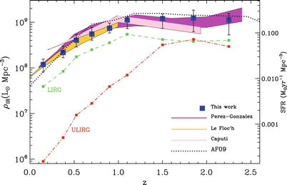
Fig. 9.44
From the luminosity functions shown in
Fig. 9.43,
the comoving total infrared luminosity density is obtained, and
plotted as a function of redshift (left axis); on the right axis,
the luminosity density is translated into an estimate of the
corresponding star-formation rate density. Results from different
studies are combined here, and they mutually agree quite well. The
green and red dashed curves show the contribution
to the luminosity density coming from galaxies with L IR ≥ 1011
L ⊙ (LIRGs) and
those with L
IR ≥ 1012 L ⊙ (ULIRGs). Source:
G. Rodighiero et al. 2010, Mid- and far-infrared luminosity functions and
galaxy evolution from multiwavelength Spitzer observations up to
z ∼ 2. 5, A&A 515, A8, p. 18, Fig. 16. ©ESO. Reproduced
with permission
Mid-IR luminosity
function. Whereas the rest-frame UV-radiation indicates the
level of star formation which is unobscured by dust, it misses
those star-forming galaxies which are heavily obscured by dust.
Their activity can best be seen in the rest-frame mid- and far-IR.
At a fixed wavelength, the emitted flux depends on the amount of
heat absorbed by the dust—and reradiated as thermal dust
emission—and on the dust temperature. Therefore, the most reliable
indicator of the obscured star formation rate is the bolometric
infrared luminosity. Whereas this is not directly observable—the
combination of sensitivity and field-of-view of far-IR detectors
allows one to study only relatively bright objects—the combination
of observations at optical, near-IR and mid-IR can be used to
estimate the dust temperature and thus to derive the bolometric IR
luminosity from the Spitzer 24 μm data and the derived dust
temperature.
The corresponding evolution of the IR luminosity
function is shown in Fig. 9.43 for several redshift bins. Although for
the higher-redshift bins only the highest luminosity sources can be
observed, the figure shows a dramatic evolution towards higher
redshift: The number density of luminous sources increases by a
large factor compared to the local one. The trend is similar to
that shown in Fig. 9.42 for the K-band luminosity function, but
even stronger. The increase of very strongly star-forming galaxies
with redshift is stronger than that with large stellar masses.
Combined with the evolution of largely unobscured star-formation,
shown in Fig. 9.41, we therefore conclude that the
star-forming activities had a much higher level in earlier epochs
of cosmic evolution than it has today. We will come back to this
point in more detail in Sect. 9.6
Integrating the Schechter function fits shown in
Fig. 9.43
over luminosity, one obtains the total infrared luminosity emitted
per unit comoving volume. The redshift evolution of this IR
luminosity density is shown in Fig. 9.44. It must be pointed
out that these estimates carry quite some uncertainty, since they
require the extrapolation of the luminosity function to much
fainter levels than those where data are available. In particular,
the faint-end slope of the Schechter function is not at all well
determined at high redshifts. Therefore, the detailed behavior of
the luminosity density beyond z ∼ 1 may be slightly different from
what is shown in the figure. However, the contribution of the LIRGs
(defined as L ≥ 1011 L ⊙) and ULIRGs
(L ≥ 1012
L ⊙) to the
luminosity density, also shown in Fig. 9.44, is much better
determined. While the IR luminosity density increases by a
factor ∼ 20 between today and z ∼ 1, and stays roughly constant up to
z ∼ 2. 5, the contribution
from ULIRGs increases by at least a factor 100 over the same
redshift range.
These results were confirmed with Herschel
blank-field surveys, centered on fields for which multi-band
observations were previously available (such as the GOODS fields or
COSMOS). Observing in the far-IR, Herschel samples the peak of the
spectral energy distribution directly, and fewer extrapolations are
necessary to derive the bolometric infrared luminosity than
required for using Spitzer data only. The analysis of the Herschel
data showed that the evolution of the IR luminosity function with
redshift is indeed dramatic. If one parametrizes the luminosity
function as a Schechter function, the characteristic luminosity
L ∗ in the
infrared increases like (1 + z)3. 5 for 0 ≲ z ≲ 2, and ∝ (1 + z)1. 6 for 2 ≲ z ≲ 4. The normalization Φ ∗ of the Schechter
function decreases with redshift, with  for
0 ≲ z ≲ 1. 1, and
for
0 ≲ z ≲ 1. 1, and
 for 1. 1 ≲ z ≲ 4. In agreement with the results
shown in Fig. 9.43, the comoving space density of very
IR-luminous sources increases by huge factors from today to higher
redshifts, before it starts to decline beyond redshift z ∼ 3.
for 1. 1 ≲ z ≲ 4. In agreement with the results
shown in Fig. 9.43, the comoving space density of very
IR-luminous sources increases by huge factors from today to higher
redshifts, before it starts to decline beyond redshift z ∼ 3.
for
0 ≲ z ≲ 1. 1, and
for 1. 1 ≲ z ≲ 4. In agreement with the results
shown in Fig. 9.43, the comoving space density of very
IR-luminous sources increases by huge factors from today to higher
redshifts, before it starts to decline beyond redshift z ∼ 3.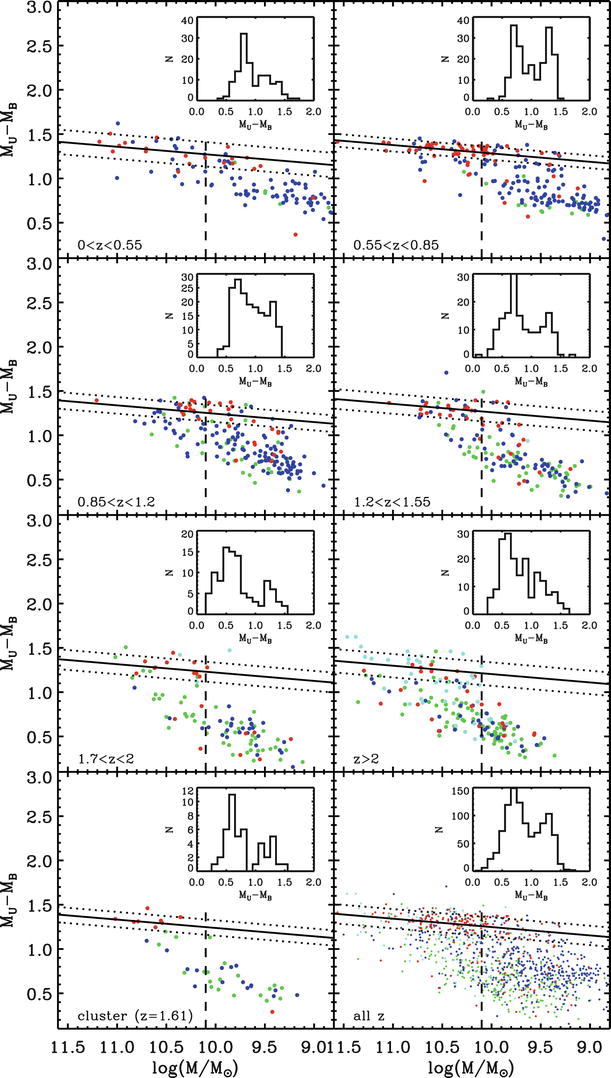
Fig. 9.45
The restframe U − B color, as a function of stellar mass,
in six redshifts bins, as indicated in the six top panels. The two bottom panels show the
color-stellar mass diagram for a proto-cluster at z = 1. 61, and the color-mass relation
for all galaxies of the sample, irrespective of redshift. The
straight line in each panel
presents a fit to the red sequence, and the vertical dashed line indicates the
completeness limit of the galaxy sample taken from the GMASS
(Galaxy Mass Assembly ultradeep Spectroscopic Survey) project, in
combination with multi-band photometry from optical to mid-infrared
wavelengths in the GOODS-South field. The available high-resolution
HST imaging allowed a morphological classification of the galaxies,
according to which the symbols are color coded: early types
(red), spirals
(blue), irregulars
(green), whereas
cyan symbols are galaxies
which are undetected in the optical bands and hence cannot be
classified morphologically; those latter galaxies can appear only
at the higher redshifts. The small
inset in each panel shows the histogram of the color
distribution. Source: P. Cassata et al. 2008,
GMASS ultradeep spectroscopy of
galaxies at z ∼ 2. III. The
emergence of the color bimodality at z ∼ 2, A&A 483,
L39, p. L40, Fig. 1. ©ESO. Reproduced with permission

Fig. 9.46
Five z ∼ 2 galaxies from the CANDLES survey.
Shown on the left is an IJH
color composite of the galaxy, which corresponds to the restframe
UV-to-optical wavelength range. The surface brightness in two
filters centered on 0.85 and 1. 6 μm is shown in the next two columns. The fourth column displays the estimated
U − V restframe color, and the right column is the estimated stellar
surface mass density. Source: S. Wuyts et al. 2012,
Smooth(er) Stellar Mass Maps in
CANDELS: Constraints on the Longevity of Clumps in High-redshift
Star-forming Galaxies, ApJ 753, 114, p 6, Fig. 2. ©AAS.
Reproduced with permission
9.4.2 The color-magnitude distribution
The color bimodality, seen prominently in the
local population of galaxies (see Sect. 3.1.3), has been in place at least
since z ∼ 2. As shown in
Fig. 9.45,
using spectroscopy of a 4. 5 μm-flux limited sample of galaxies in
the GOODS South field, for which deep photometry is available over
a wide range of optical and infrared bands (including HST and
Spitzer), the color bimodality can be clearly seen in all redshift
intervals.
At even higher redshift, the sample of galaxies
on the red sequence gets increasingly contaminated by dusty
star-forming galaxies. However, one can account for this reddening
and obtain dust-corrected colors for those galaxies. After this
correction, the color bimodality can be detected out to redshifts
z ∼ 3, implying that
already at young cosmic epochs, galaxies with an old stellar
population coexisted with those which actively formed stars.
Accordingly, the red sequence was formed early on, as can also be
seen in Fig. 9.45.
This observational results implies that even at
high redshifts, a large fraction of galaxies exists with a
passively evolving stellar population. Whereas the star-forming
galaxies—LBGs and SMGs—are the more spectacular objects at these
high redshifts, many galaxies had formed their stars at even
earlier epochs. From what we mentioned above—see, e.g.,
Fig. 9.42—the
more massive galaxies seem to conclude most of the built-up of
their stellar population at the highest redshifts. In parallel with
the color-magnitude relation, also the local color-density relation
was in place at least since z ∼ 1.
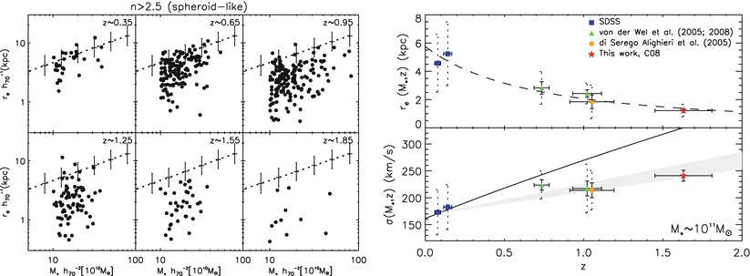
Fig. 9.47
Left
panel: The effective radius (i.e., the radius within which
half the light is emitted) versus stellar mass of galaxies with
Sérsic index n > 2. 5,
representing early-type galaxies, for different redshifts. In each
panel, the corresponding relation obtained in the local Universe is
shown as solid curve with
estimated uncertainties shown as error bars. Right panel: The mean effective radius
(top) and velocity
dispersion (bottom) as a
function of redshift, for galaxies with stellar masses of
M
∗ ∼ 1011 M ⊙. The solid curve and grey band in the bottom panel shows two different models
for the evolution of spheroidals. Source: Left: I. Trujillo et al. 2007,
Strong size evolution of the most
massive galaxies since z ∼ 2, MNRAS 382, 109, p. 115,
Fig. 7. Reproduced by permission of Oxford University Press on
behalf of the Royal Astronomical Society. Right: A.J. Cenarro &
I. Trujillo 2009, Mild
Velocity Dispersion Evolution of Spheroid-Like Massive Galaxies
Since z ∼ 2, ApJ 696, L43, p. L46, Fig. 2. ©AAS. Reproduced
with permission
9.4.3 The size and shape of high-redshift galaxies
The fact that the population of galaxies evolves
strongly with redshift raises the expectation that the galaxies at
high redshift are different from those in the local Universe. Here
we will point out some of these differences.
The Hubble
sequence and galaxy morphology. The majority of present day
massive galaxies fall onto the morphological Hubble sequence
(Fig. 3.2). In addition, we have seen that
local galaxies can be classified according to their color, with
most of them being either member of the red sequence or the blue
cloud, as seen in Fig. 3.38, with a tight correspondence
between the Hubble classification and the galaxy color and
morphological parameters, such as the Sérsic index.
The situation at high redshifts is quite
different. At z ≳ 3, most
of the galaxies are strongly star forming, with a rather small
population of quiescent galaxies. The star-forming objects do not
appear at all to have a regular morphology, rather, they are
irregular, or clumpy. In Fig. 9.46, five z ∼ 2 galaxies are shown as a IJH-color
composite image. The irregular, knotty structure is easily seen,
and many of the bright knots are clearly well separated from the
center of the galaxy—these galaxies do not appear to fall on the
Hubble sequence. These clumps have a characteristic size
of ∼ 1 kpc, and they seem to be projected onto a kind of disk
galaxy. In fact, using high angular resolution integral field
spectroscopy, the rotation of several of such z ∼ 2 galaxies could clearly be shown.
But these disk are not rotating quietly, in contrast to local disk
galaxies, they have a very large velocity dispersion. This fact
renders the interpretation of the observed velocity field in terms
of Kepler rotation more complicted than for thin, kinematically
cold disk galaxies.
However, we should keep in mind that the
rest-frame UV light distribution is dominated by star-forming
regions. The second and third column in Fig. 9.46 show the surface
brightness of these galaxies in two different filters separately,
and an estimate of the rest-frame U − V color is shown in the fourth column.
We can see that the clumps are typically significantly bluer than
the rest of the galaxy, and hence their stellar population has a
younger age than the underlying disk. The stellar mass contained in
the clumps make a 7 % contribution to the total stellar mass of the
galaxy, but they contribute about 20 % to the star-formation rate.
Finally, the right column shows the reconstructed stellar surface
mass density. Now the picture is a quite different one: the stellar
mass is seen to be centrally concentrated, and no prominent
off-center clumps are present.
Quiescent galaxies become more abundant towards
lower redshift; it is estimated that the stellar mass contained in
quiescent objects increases by a factor ∼ 15 between redshifts 3
and 1, and by another factor of ∼ 3 from there until today. In
other word, the number of passive red galaxies has at least doubled
since z = 1 until today, so
that many of the early-type galaxies in the current Universe
arrived on the red sequence at rather low redshift. For
z > 2, peculiar galaxies
dominate the galaxy population, with some quiescent, spheroidal
galaxies already present then, but a negligible disk population. At
a redshift around z ∼ 2,
the abundance of spheroidal and disk galaxies together start to
overtake the peculiar population, where this redshift depends on
mass: at higher mass, the fraction of Hubble sequence-like galaxies
is higher than at lower masses, indicating that they finish their
morphological evolution earlier. Thus, starting from z ∼ 2, the Hubble sequence is gradually
built up.
Size
evolution. Red, quiescent galaxies at z ∼ 2 not only have a regular
morphology compared to the clumpy star-forming galaxies, but they
also are more massive and more compact. The latter aspects can be
seen in Fig. 9.47, where in the left panel the effective
radius is plotted as a function of stellar mass, for galaxies with
Sérsic index n > 2. 5
and different redshift bins. Compared to the local population of
early-type galaxies, higher-redshift spheroidal galaxies are
significantly smaller at fixed stellar mass. The effective radius
as a function of redshift, for a fixed stellar mass, is shown in
the upper panel on the right. The size evolution is fitted with a
power law of the form  . The
decrease in radius at fixed stellar mass by a factor of ∼ 3 at
z ∼ 1. 5 implies that these
galaxies have a stellar density larger by a factor ∼ 30 than
present day early-type galaxies—these high-redshift galaxies are
very different from the current population. The higher density also
implies a larger velocity dispersion, which is indeed observed, as
seen in the bottom panel on the right in Fig. 9.47.
. The
decrease in radius at fixed stellar mass by a factor of ∼ 3 at
z ∼ 1. 5 implies that these
galaxies have a stellar density larger by a factor ∼ 30 than
present day early-type galaxies—these high-redshift galaxies are
very different from the current population. The higher density also
implies a larger velocity dispersion, which is indeed observed, as
seen in the bottom panel on the right in Fig. 9.47.Indeed, such compact galaxies are very rare in
the local Universe—that means that the typical z ∼ 2 quiescent galaxy must have
evolved significantly to fit into the local zoo of galaxies. Two
principal possibility for this evolution exist: either the galaxies
grow in size, at fixed stellar mass, or they accumulate more mass
in their outer parts, thereby growing in mass and in size, such
that they become less compact in this evolution. The latter
possibility seems to be closer to the truth, as shown by
simulations. Minor merging processes can yield an evolution that is
compatible with the observational finding. Thus, early-type
galaxies seem to grow inside-out: Their inner region was in place
at earlier epochs, their outer parts were added lateron by merging
processes.
9.4.4 The interstellar medium
The interstellar medium in high-redshift galaxies
differs from that of local galaxies in a number of properties, of
which we mention just a few here.
Metallicity. For local galaxies, there is
a clear trend of increasing metallicity with increasing mass, as
shown in Fig. 3.40. A similar trend is observed
for Lyman-break galaxies at z ∼ 2, except that the normalization of
the mass-metallicity relation is smaller by a factor ∼ 2, as can be
seen in Fig. 9.48. Of course, this result does not come
unexpectedly, since at earlier redshifts, there was less time to
enrich the ISM.
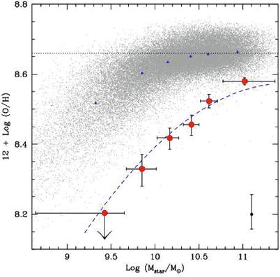
Fig. 9.48
The metallicity of UV-selected z ∼ 2 galaxies, as a function of
stellar mass (big dots with
error bars). For comparison, the mass-metallicity relation for
local SDSS galaxies is shown, as in Fig. 3.40. Whereas the shape of the
mass-metallicity relation is similar at both redshifts, the
normalization is lower by about a factor of two at z ∼ 2. Source: D.K. Erb et
al. 2006, The
Mass-Metallicity Relation at z ≳ 2, ApJ 644, 813, p. 819,
Fig. 3. ©AAS. Reproduced with permission
Whereas the metallicity of star-forming galaxies
is lower than at the current epoch, at least some galaxies managed
to enrich their ISM to about Solar values, as can be inferred from
the metallicity of the broad-line emitting gas in high-redshifts
QSOs. Not only did these objects form supermassive black holes with
M
• ≳ 109 M ⊙, but the chemical
evolution in these objects was already mature at a small cosmic
age. Of course, luminous high-z QSOs are rare and most likely
populate the most massive halos available at these epochs.
Gas
content. Second, the high star-formation rate implies the
presence of a large reservoir of gas. As we have seen, in the
current Universe the gas-mass fraction of even late-type spiral
galaxies is below ∼ 30 %;
in contrast to that, high-z
star-forming galaxies typically have a gas-mass fraction
of ∼ 50 %.
Instead of considering the absolute
star-formation rate  , it is often meaningful to study the
specific star-formation rate,
, it is often meaningful to study the
specific star-formation rate,  , i.e., the star-formation rate
per unit stellar mass. This quantity has the units of an inverse
time: the inverse of the specific star-formation rate is the time
it would take to built up the stellar mass present if the
star-formation rate would be a constant. At a fixed gas-mass
fraction, this time is very similar to the time-scale on which all
the gas in a galaxy is transformed into stars. The specific
star-formation rate of Lyman-break galaxies increases by a
factor ∼ 10 between the current epoch and z ∼ 1. 5, but then appears to stay
remarkably constant out to z ∼ 7 (where, of course, the results at
the highest redshifts carry an appreciable uncertainty).
, i.e., the star-formation rate
per unit stellar mass. This quantity has the units of an inverse
time: the inverse of the specific star-formation rate is the time
it would take to built up the stellar mass present if the
star-formation rate would be a constant. At a fixed gas-mass
fraction, this time is very similar to the time-scale on which all
the gas in a galaxy is transformed into stars. The specific
star-formation rate of Lyman-break galaxies increases by a
factor ∼ 10 between the current epoch and z ∼ 1. 5, but then appears to stay
remarkably constant out to z ∼ 7 (where, of course, the results at
the highest redshifts carry an appreciable uncertainty).
, it is often meaningful to study the
specific star-formation rate, , i.e., the star-formation rate
per unit stellar mass. This quantity has the units of an inverse
time: the inverse of the specific star-formation rate is the time
it would take to built up the stellar mass present if the
star-formation rate would be a constant. At a fixed gas-mass
fraction, this time is very similar to the time-scale on which all
the gas in a galaxy is transformed into stars. The specific
star-formation rate of Lyman-break galaxies increases by a
factor ∼ 10 between the current epoch and z ∼ 1. 5, but then appears to stay
remarkably constant out to z ∼ 7 (where, of course, the results at
the highest redshifts carry an appreciable uncertainty).Dust. The
fact that the far-IR emission is the best indicator for star
formation already indicates that these galaxies must contain a
significant dust abundance. The dust temperature, which determines
the spectral shape in the far-IR, can vary in these dusty galaxies
over quite a substantial range, 25 K ≲ T d ≲ 65 K, as determined
recently from Herschel observations. The impact of the dust
temperature on the spectral shape means that single-band selection,
e.g., the flux at 850 μm, can bias against objects with hotter dust
temperature.
Whereas most of the properties of z ∼ 6 QSOs are indistinguishable from
those of low-redshift QSOs, there are signs that they differ in
their near-IR properties. In local QSOs, the UV/optical continuum
emission is believed to be mainly due to the accretion disk,
whereas the near-IR radiation is due to hot dust, heated by the
AGN. The ratio of NIR-to-optical luminosity of z ≲ 5 QSOs is confined to a rather
small range around ∼ 1. In a sample of 21 z ∼ 6 QSOs, there are two sources
without detected NIR emission, yielding an upper limit to the
NIR-to-optical flux ratio that is one order of magnitude smaller
than the value typically observed. Using a control sample of more
than 200 lower-z QSOs, not
a single one has this flux ratio as low as the sources at
z ∼ 6. The lack of
detectable NIR emission can be attributed to the lack of dust in
these systems.
A clue for the origin of this lack of dust is
obtained from a second finding: the NIR-to-optical flux ratio for
lower-z QSOs shows no
correlation with the SMBH mass as estimated from the width of broad
emission lines. In contrast to that, there seems to be a strong
dependence of this flux ratio on the SMBH mass in the sample of
z ∼ 6 QSO, in that the
ratio increases with increasing M •. A simple interpretation
of this result could be that these high-redshift QSOs were able to
build up their SMBH and the corresponding accretion disk, but that
they were unable yet to form large masses of dust. The larger
M •, the more
evolved is the AGN, and the more dust was created. It remains to be
seen whether this interpretation survives further observational
tests.
9.5 Background radiation at smaller wavelengths
The cosmic microwave background (CMB) is a
remnant of the early hot phase of the Universe, namely thermal
radiation from the time before recombination. As we extensively
discussed in Sect. 8.6, the CMB contains a great deal
of information about our Universe. Therefore, one might ask whether
background radiation also exists in other wavebands, which then
might be of similar value for cosmology. The neutrino background
that should be present as a relic from the early epochs of the
Universe, in the form of a thermal distribution of all three
neutrino families with T ≈ 1. 9 K (see Sect. 4.4.3), is likely to remain
undiscovered for quite some time due to the very small cross
section of these low-energy neutrinos.
Indeed, apparently isotropic radiation has been
found in wavelength domains other than the microwave regime
(Fig. 9.49).
In this figure, the background radiation measured as ν I ν is plotted against wavelength,
so that the curve shows the intensity per logarithmic frequency
interval. Following the terminology of the CMB, these are called
background radiation as well. However, the name should not imply
that it is a background radiation of cosmological origin, in the
same sense as the CMB. From the thermal cosmic history (see
Sect. 4.4), no optical or X-ray radiation
is expected from the early phases of the Universe. Hence, for a
long time it was unknown what the origin of these different
background components may be.
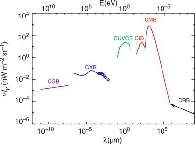
Fig. 9.49
Spectrum of cosmic background radiation,
plotted as ν I
ν versus
wavelength. Besides the CMB, background radiation exists in the
radio domain (cosmic radio background, CRB), in the infrared (CIB),
in the optical/UV (CUVOB), in the X-ray (CXB), and at gamma-ray
energies (CGB). With the exception of the CMB, all of these
backgrounds can be understood as a superposition of the emission
from discrete sources. Furthermore, this figure shows that the
energy density in the CMB exceeds that of other radiation
components, as was assumed when we considered the radiation density
in the Universe in Chap. 4. Source: M.G. Hauser &
E. Dwek 2001, The Cosmic
Infrared Background: Measurements and Implications,
ARA&A 39, 249, Fig. 1. Reprinted, with permission, from the
Annual Review of Astronomy &
Astrophysics, Volume 39 ©2001 by Annual Reviews www.annualreviews.org
At first, the early X-ray satellites discovered a
background in the X-ray regime (cosmic X-ray background, CXB).
Later, the COBE satellite detected an apparently isotropic
radiation component in the FIR, the cosmic infrared background
(CIB).

Fig. 9.50
The spectrum of the cosmic infrared
background. The black
arrows show the lower bound on the CIB, which is obtained
from individually observed sources in these wavebands, i.e., by
integrating the source counts at these frequencies up to the
completeness limit. Blue
arrows are lower bounds based on an extrapolation of the
source counts to lower fluxes. The magenta arrows are upper limits,
obtained from the Voyager spacecraft. The filled circles and stars with error bars are estimates,
obtained with HST and several NIR instruments, as indicated. The
solid magenta line presents
an upper limit, obtained from the transparency of the Universe for
very high-energy gamma rays with respect to electron-positron pair
production (see Sect. 9.5.2); note that this upper limit is very
close to the lower bound obtained from source counts. The
open squares are estimates
of the CIB from IRAS and the DIRBE instrument onboard COBE, while
the solid curve at the
longest wavelengths is the spectral estimate from FIRAS. Source:
H. Dole et al. 2006, The
cosmic infrared background resolved by Spitzer. Contributions of
mid-infrared galaxies to the far-infrared background,
A&A 451, 417, p. 426, Fig. 11. ©ESO. Reproduced with
permission
In the present context, we simply denote the flux
in a specific frequency domain, averaged over sky position at high
Galactic latitudes, as background radiation. Thus, when talking
about an optical background here, we refer to the sum of the
radiation of all galaxies and AGNs per solid angle. The
interpretation of such a background radiation depends on the
sensitivity and the angular resolution of the telescopes used.
Imagine, for instance, observing the sky with an optical camera
that has an angular resolution of only one arcminute. A relatively
isotropic radiation would then be visible at most positions in the
sky, featuring only some very bright or very large sources. Thus,
the background can be decomposed into a ‘resolved’ component, which
can be attributed to individually identified sources, and the
unresolved component. On improving the angular resolution, more and
more individual sources become visible, so that a larger fraction
of the background radiation is resolved. At optical wavebands, the
Hubble Deep Fields have resolved essentially all of the background
into individual sources. In analogy to this, one may wonder whether
the CXB or the CIB can likewise be understood as a superposition of
radiation from discrete sources.
9.5.1 The IR background
The first point to note from Fig. 9.49 is the relatively
flat energy distribution between the UV- and the mm-regime. Since
both, the UV-radiation and the far-IR radiation originate almost
entirely from star-formation, the flat energy distribution implies
that essentially half of the energetic photons emitted from
newly-formed stars are absorbed by dust and reradiated in the FIR.
Hence, estimates of the star-formation activity from UV-flux alone
will on average be biased low by ∼ 50 %.
Absolute measurements of the intensity of the
background radiation are difficult to obtain, since it requires an
absolute calibration of the instruments. The filled circles and
stars with error bars in Fig. 9.50 show estimates of the background radiation
level in the optical and near-IR. The black arrows show the
integrated light of all sources which are detectable in the deepest
observations with HST; within the error bars of the estimated level
of the background radiation, these results are compatible with the
background being solely due to the superposition of individual
optical and near-IR sources, i.e., galaxies and (to a lesser
degree) AGNs.
Observations of background radiation in the
infrared are very difficult to accomplish, in particular due to the
thermal radiation from the instruments and the zodiacal light.
However, the DIRBE and FIRAS instruments onboard COBE provided a
measurement (in fact, the detection) of the CIB. The question now
is whether the CIB can be understood as well as being due solely to
individual sources.
Confusion
limit. Since mid- and far-IR observations are only possible
from space, finding the answer to that question is challenging.
Infrared observatories in space have a rather small aperture which,
together with the long wavelength, yields a rather large
point-spread function (PSF). This implies that when one observes to
low flux limits, where the mean angular separation of sources on
the sky becomes comparable to the size of the PSF, these sources
can not be separated. This yields a lower flux limit for the
detection of individual sources, called the confusion limit. The
smaller the telescope, the shallower is the confusion limit
reached. For example, the flux limit down to which individual
sources could be identified with the Spitzer satellite at 160 μm
corresponds to only 7 % of the CIB at this wavelength. The much
larger mirror on the Herschel satellite lowered the confusion limit
such that individual sources can be identified which account for
about 52 % of the CIB. Going to larger wavelength, the confusion
limit is even more severe.
Stacking.
However, one can dig deeper into the source counts with a technique
called stacking. Taking the position of sources detected at some
smaller wavelength (where the confusion limit is fainter), and
adding up the flux in the longer wavelength band around all these
positions, one obtains the mean long-wavelength flux of these
sources. With this method, one will miss all fainter sources which
do not have a detected counterpart in the short-wavelength input
catalog, so that wavelength should be selected carefully. Given the
characteristic spectrum of FIR-bright sources shown in
Fig. 9.30,
one expects that most of the sources radiating in the FIR will have
an appreciable flux at 24 μm. Since Spitzer was particularly
sensitive at this wavelength, the corresponding source catalog is
best for a stacking analysis. Furthermore, if the redshifts of the
sources selected at 24 μm is known, the stacking analysis can be
used to determine the redshift distribution of the contributions to
the CIB in the FIR. With stacking, the source counts can be
followed to about three times lower flux than the confusion limit
of individual sources permits.
The state of the art is defined by deep fields
observed with the Herschel observatory, owing to its large aperture
and sensitive instrumentation. From observing the well-studied
GOODS, COSMOS, and ECDFS fields, where detailed multi-waveband data
from other observatories are available, Herschel was able to
attribute between 65 and 89 %, depending on wavelength, of the
estimated CIB level between 100 and 500 μm to resolved sources or
sources seen at 24 μm. A moderate extrapolation of the source
counts to fainter flux limits then shows that the bulk, if not all,
of the CIB comes from galaxies or AGNs.
In addition, the redshift distribution of the CIB
could be determined. At wavelengths below ∼ 160 μm, more than half
of the CIB radiation comes from sources at z < 1, whereas at longer wavelength,
the source distribution shifts to increasingly higher redshifts.
The major fraction of the CIB is due to galaxies with infrared
luminosities in the range 1011 to 1012
L ⊙, i.e., due
to LIRGs.
9.5.2 Limits on the extragalactic background light from γ-ray blazars
The added flux of sources, either individually
detected or obtained from a stacking analysis, yields a lower limit
to the extragalactic background light, which in the UV, optical and
near-IR regime is smaller than estimates of the total intensity of
the background, as seen in Fig. 9.50, although these latter measurements have
fairly larger error bars. Hence, the question arises whether there
are other sources of the background light not identified as
individual sources—for example, very low surface brightness
galaxies that could escape detection. In fact, this question can be
answered from observations of blazars (see Sect. 5.2.6) at energies in the GeV and
TeV regime, as will be described next.
Attenuation
of γ -rays: Condition for pair production.
High-energy photons from distant sources propagate through the
extragalactic background radiation field. If the photon energy is
high enough, then by colliding with one of the background photons,
it may produce an  -pair, in which case it
does not reach the Earth. Thus, this pair production attenuates the
flux from the source.
-pair, in which case it
does not reach the Earth. Thus, this pair production attenuates the
flux from the source.
-pair, in which case it
does not reach the Earth. Thus, this pair production attenuates the
flux from the source.In order for pair production to occur, the
product of the energies of the background-light photon
(ε) and the photon from the
source (E γ ) must be sufficiently high. If
the two photons propagate in opposite direction (head-on
collision), then the threshold condition is ε E γ > (m e c 2)2. In
general, if the photon directions enclose an angle θ, this gets modified to
 We see that the threshold energy is smallest for head-on
collisions, where θ = π. The cross-section for this process
is small for photon energies very close to the threshold, reaches
its maximum at about twice the threshold energy (9.3), and decreases again
for larger energies. At the maximum of the cross-section, the
relation between the two photon energies can be written in
practical units,
We see that the threshold energy is smallest for head-on
collisions, where θ = π. The cross-section for this process
is small for photon energies very close to the threshold, reaches
its maximum at about twice the threshold energy (9.3), and decreases again
for larger energies. At the maximum of the cross-section, the
relation between the two photon energies can be written in
practical units,

(9.3)
(9.4)
from which we see that for the attenuation of TeV
photons, extragalactic background photons in the near-IR are most
efficient, whereas radiation in the tens-of-GeV-regime can be
attenuated by UV-photons.

Fig. 9.51
Top
left: Model of the extragalactic background light, at three
different redshifts. The high-amplitude peak at long wavelengths is
the CMB and thus shows the evolution of the Planck spectrum with
redshift. Top right: The
proper photon number density per logarithmic energy interval, for
the same three redshifts. Bottom
left: The optical depth τ γ γ (E γ , z) for pair production, as a function
of the γ-ray energy.
Bottom right: The
attenuation factor exp[−τ
γ γ
(E γ , z)] as a function of the γ-ray energy. Source: E. Dwek
& F. Krennrich 2012, The
Extragalactic Background Light and the Gamma-ray Opacity of the
Universe, arXiv:1209.4661, Fig. 12. Reproduced by permission
of the author
Optical
depth. In order to derive the efficiency of the attenuation,
one needs to calculate the optical depth τ γ γ (E γ , z), which depends on the energy of the
γ-ray and the source
redshift. To obtain τ
γ γ
(E γ , z), the pair-production cross section
needs to be integrated along the line-of-sight to the source,
multiplied by the spectral energy density of the background
radiation; for this, the redshift evolution of the background
radiation needs to be accounted for. Since the extragalactic
background light can be observed only at the current redshift, one
needs to model its redshift evolution, based on what is known about
the source population. A particular model is shown in the top left
panel of Fig. 9.51, which also includes the CMB, and the
corresponding photon number density per logarithmic photon energy
interval is shown in the top right panel. Based on the background
light model, the optical depth for pair production can be
calculated, which is shown in the bottom left panel of the same
figure. τ γ γ (E γ , z) is a strong function of both, the
γ-ray energy and the
redshift. The plateau in τ
γ γ at
energies ∼ 2 TeV is due to the minimum of the background radiation
spectrum at ∼ 10 μm.
The observed flux S obs(E γ ) is related to the intrinsic
(i.e., non-attenuated) flux S int(E γ ) by
![$$\displaystyle{ S_{\mathrm{obs}}(E_{\gamma }) = S_{\mathrm{int}}(E_{\gamma })\,\exp [-\tau _{\gamma \gamma }(E_{\gamma },z)]\;, }$$](A129044_2_En_9_Chapter_Equ5.gif) where the attenuation factor
where the attenuation factor  is plotted in
the bottom right panel of Fig. 9.51. We can see that the attenuation factor
has a very steep decline with photon energy; for example, based on
this model we would not expect to see 20 TeV photons from any
source at z ≳ 0. 1. This
steep, exponential decline implies that the attenuation factor is
very sensitive to the model of the extragalactic background light;
conversely, if observations yield constraints on the attenuation
factor, then strong constraints on the background light can be
obtained, at wavelengths depending on the detection of the
attenuation, according to (9.4).
is plotted in
the bottom right panel of Fig. 9.51. We can see that the attenuation factor
has a very steep decline with photon energy; for example, based on
this model we would not expect to see 20 TeV photons from any
source at z ≳ 0. 1. This
steep, exponential decline implies that the attenuation factor is
very sensitive to the model of the extragalactic background light;
conversely, if observations yield constraints on the attenuation
factor, then strong constraints on the background light can be
obtained, at wavelengths depending on the detection of the
attenuation, according to (9.4).
(9.5)
is plotted in
the bottom right panel of Fig. 9.51. We can see that the attenuation factor
has a very steep decline with photon energy; for example, based on
this model we would not expect to see 20 TeV photons from any
source at z ≳ 0. 1. This
steep, exponential decline implies that the attenuation factor is
very sensitive to the model of the extragalactic background light;
conversely, if observations yield constraints on the attenuation
factor, then strong constraints on the background light can be
obtained, at wavelengths depending on the detection of the
attenuation, according to (9.4).Observational
constraints on the attenuation. As mentioned in
Sect. 5.5.4, blazars can emit at GeV and
TeV energies, most likely caused by their jet pointing towards us.
The Fermi Gamma-Ray Space Telescope, operating in the energy range
between 200 MeV and 300 GeV, and the air Cherenkov observatories
H.E.S.S., MAGIC and VERITAS, observing in the range
between ∼ 50 GeV and 100 TeV, have detected more than 1000 blazars
in the GeV-range and more than 30 at TeV energies. Whereas blazars
in the GeV-range are observed out to redshifts z ≥ 1, essentially all the TeV blazars
are at low redshift, most of them having z ≲ 0. 2. This is indeed what one
expects, based on the results in Fig. 9.51.7 In principle, these observations of
the spectral energy distribution could be used to determine the
attenuation factor; however, in order to employ (9.5), one needs some
knowledge about the intrinsic flux distribution S int(E γ ).
There are various ways how realistic estimates
for τ γ γ can be obtained from the
observations. The first of these is to base the intrinsic flux
distribution on models of the γ-ray emission, and constrain these
models by observations at somewhat lower photon energies. However,
the models are sufficiently uncertain to preclude very accurate
predictions, and thus the corresponding results on τ γ γ are correspondingly
uncertain. Second, since the relativistic electrons responsible for
the inverse Compton effect that presumably causes the γ-ray emission, are expected to result
from acceleration by shock fronts, as mentioned in
Sect. 5.1.3, the slope of the electron
distribution can not be arbitrarily flat, and thus the resulting
inverse Compton radiation is also limited in slope; in the notation
of Sect. 5.1.3, s ≳ 2 and thus α ≳ 0. 5. Assuming this value of the
spectral index as a limit for the intrinsic flux distribution, the
observed energy distribution can be translated into upper bounds on
the attenuation. An even weaker assumption is used by a third
methods, where one requires that the intrinsic flux S int(E γ ) = S obs(E γ ) exp[τ γ γ (E γ , z)] does not (exponentially) increase
with photon energy, as would be the case if the background light
intensity would be overestimated.
Results.
Depending on which of these methods are used, the results will
differ slightly. A particular result is shown in Fig. 9.50, where the magenta
curve indicates the upper bound on the extragalactic background
light obtained from the high-energy observations of blazars. This
upper bound is almost coincident with the lower bound obtained from
the resolved source counts in the UV, optical and near-IR regime,
strongly arguing that there are no other significant contributions
of the background light than the observed galaxies and AGN. It thus
seems that the spectral intensity of the background light in this
spectral regime is now rather well determined. This conversely
implies that the optical depth τ γ γ is very well constrained,
which in turn allows us to derive the intrinsic flux distribution
from the observed one. In the future, this method will therefore
yield more detailed constraints on the emission mechanism for
high-energy radiation from blazars and other AGNs.
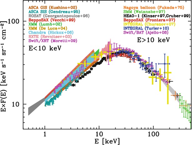
Fig. 9.52
Measurement of the cosmic X-ray background
over a wide range of photon energies, measured by different
satellites and instruments. Source: R. Gilli 2013,
The cosmic X-ray background:
abundance and evolution of hidden black holes,
arXiv:1304.3665, Fig. 1. Reproduced by permission of the
author
9.5.3 The X-ray background
The first X-ray experiment in astronomy, a
balloon flight in 1962, discovered a diffuse X-ray emission across
the sky, confirmed by the first X-ray satellites which discovered
not only a number of extragalactic X-ray sources (such as AGNs and
clusters of galaxies), but also an apparently isotropic radiation
component. The spectrum of the cosmic X-ray background (CXB) is a
very hard (i.e., flat) power law, cut off at an energy
above ∼ 40 keV, which can roughly be described by
 with E
0 ∼ 40 keV. A recent estimate of the spectrum of the CXB
is shown in Fig. 9.52. The estimates from different instruments
agree in general, though differences in the level are clearly
visible. These differences can have a number of origins, including
cosmic variance (the spectral shape of the CXB is usually
determined from rather small fields, so there could be variations
from field to field), stray light entering the telescope, and
remaining calibration uncertainties of the instruments. Together,
the CXB is known with an uncertainty of ∼ 20 %.
with E
0 ∼ 40 keV. A recent estimate of the spectrum of the CXB
is shown in Fig. 9.52. The estimates from different instruments
agree in general, though differences in the level are clearly
visible. These differences can have a number of origins, including
cosmic variance (the spectral shape of the CXB is usually
determined from rather small fields, so there could be variations
from field to field), stray light entering the telescope, and
remaining calibration uncertainties of the instruments. Together,
the CXB is known with an uncertainty of ∼ 20 %.
(9.6)
Initially, the origin of this radiation was
unknown, since its spectral shape was different from the spectra of
sources that were known at that time. For example, it was not
possible to obtain this spectrum by a superposition of the spectra
of known AGNs.
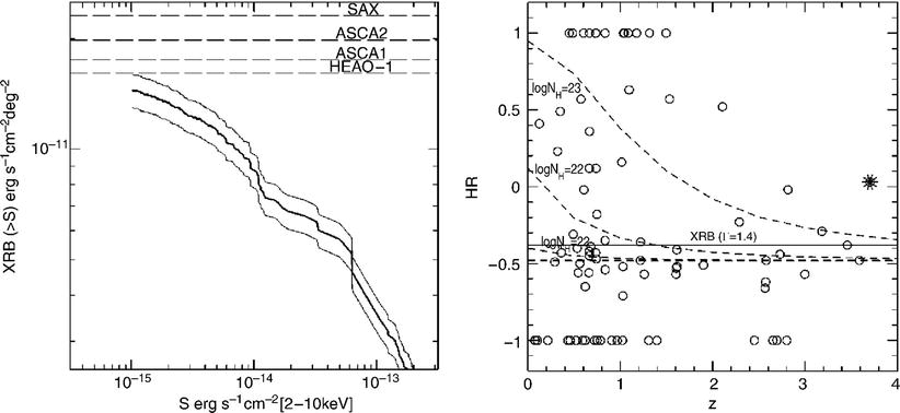
Fig. 9.53
In the left panel, the total intensity of
discrete sources with an individual flux > S in the energy range
2 keV ≤ E ≤ 10 keV is
plotted (thick curve),
together with the uncertainty range (between the two thin curves). Most of the data are from
a 3 × 10⁵ s exposure of the Chandra Deep Field. The
dashed lines show different
measurements of the CXB flux in this energy range; depending on
which of these values is the correct one, between 60 and 90 % of
the CXB in the Chandra Deep Field at this energy is resolved into
discrete sources. In the right
panel, the hardness ratio HR—specifying the ratio of photons
in the energy range 2 keV ≤ E ≤ 10 keV to those in
0. 5 keV ≤ E ≤ 2 keV,
 —is
plotted as a function of redshift, for 84 sources in the Chandra
Deep Field with measured redshifts. This plot indicates that the HR
decreases with redshift; this trend is expected if the X-ray
spectrum of the AGNs is affected by intrinsic absorption. The
dashed curves show the
expected value of HR for a source with an intrinsic power-law
spectrum I
ν
∝ ν −0. 7,
which is observed through an absorbing layer with a hydrogen column
density of N H,
by which these curves are labeled. Since low-energy photons are
more strongly absorbed by the photoelectric effect than high-energy
ones, the absorption causes the spectrum to become harder, thus
flatter, at relatively low X-ray energies. This implies an increase
of the HR (also see the bottom
panel of Fig. 6.22). This effect is smaller for
higher redshift sources, since the photon energy at emission is
then larger by a factor of (1 + z). Source: P. Tozzi et
al. 2001, New Results from
the X-Ray and Optical Survey of the Chandra Deep Field-South: The
300 Kilosecond Exposure. II., ApJ 562, 42, p. 48, 49,
Figs. 7, 9. ©AAS. Reproduced with permission
—is
plotted as a function of redshift, for 84 sources in the Chandra
Deep Field with measured redshifts. This plot indicates that the HR
decreases with redshift; this trend is expected if the X-ray
spectrum of the AGNs is affected by intrinsic absorption. The
dashed curves show the
expected value of HR for a source with an intrinsic power-law
spectrum I
ν
∝ ν −0. 7,
which is observed through an absorbing layer with a hydrogen column
density of N H,
by which these curves are labeled. Since low-energy photons are
more strongly absorbed by the photoelectric effect than high-energy
ones, the absorption causes the spectrum to become harder, thus
flatter, at relatively low X-ray energies. This implies an increase
of the HR (also see the bottom
panel of Fig. 6.22). This effect is smaller for
higher redshift sources, since the photon energy at emission is
then larger by a factor of (1 + z). Source: P. Tozzi et
al. 2001, New Results from
the X-Ray and Optical Survey of the Chandra Deep Field-South: The
300 Kilosecond Exposure. II., ApJ 562, 42, p. 48, 49,
Figs. 7, 9. ©AAS. Reproduced with permissionROSAT, with its substantially improved angular
resolution compared to earlier satellites (such as the Einstein observatory), conducted source
counts at much lower fluxes, based on some very deep images. From
this, it was shown that at least 80 % of the CXB in the energy
range between 0.5 and 2 keV is emitted by discrete sources, of
which the majority are AGNs. Hence it is natural to assume that the
total CXB at these low X-ray energies originates from discrete
sources, and observations by XMM-Newton and Chandra have confirmed
this.
However, the X-ray spectrum of normal AGNs is
different from (9.6), namely it is considerably steeper (about
S ν ∝ ν −0. 7). Therefore, if
these AGNs contribute the major part of the CXB at low energies,
the CXB at higher energies cannot possibly be produced by the same
AGNs. Subtracting the spectral energy of the AGNs found by ROSAT
from the CXB spectrum (9.6), one obtains an even harder spectrum,
resembling very closely that of thermal bremsstrahlung. Therefore,
it was supposed for a long time that the CXB is, at higher
energies, produced by a hot intergalactic gas at temperatures of
k B T ∼ 30 keV.
This model was excluded, however, by the precise
measurement of the thermal spectrum of the CMB by COBE, showing
that the CMB has a perfect blackbody spectrum. If a postulated hot
intergalactic gas were able to produce the CXB, it would cause
significant deviations of the CMB from the Planck spectrum, namely
by the inverse Compton effect (the same effect that causes the SZ
effect in clusters of galaxies—see Sect. 6.4.4). Thus, the COBE results
clearly ruled out this possibility.
Deep observations with Chandra and XMM (e.g., in
the CDFS shown in Fig. 9.14) have finally resolved most of the CXB
also at higher energies, as seen in Fig. 9.53. From source counts
performed in such fields, more than 75 % of the CXB in the energy
range of 2 keV ≤ E ≤ 10 keV
could be resolved into discrete sources. Again, most of these
sources are AGNs, but typically with a significantly harder (i.e.,
flatter) spectrum than the AGNs that are producing the low-energy
CXB. Such a flat X-ray spectrum can be produced by photoelectric
absorption of an intrinsically steep power-law spectrum, where
photons closer to the ionization energy are more efficiently
absorbed than those at higher energy. According to the
classification scheme of AGNs discussed in Sect. 5.5, these are Type 2 AGNs, thus
Seyfert 2 galaxies and QSOs with strong intrinsic self-absorption.
We should recall that Type 2 QSOs have only been detected by
Chandra—hence, it is no coincidence that the same satellite has
also been able to resolve the high-energy CXB.
However, at even higher energies most of the CXB
was still unaccounted for—even the observed Type-2 AGNs could not
account for it. It thus seems that there is a population of sources
in the Universe which dominate the X-ray emission at high energies,
still escape the observations at low X-ray frequencies. These could
be heavily obscured AGNs, where only the hard X-rays manage to
escape the emitting region. With the X-ray telescope onboard the
Swift satellite, a significant number of such heavily obscured AGNs
were found. Their estimated number density, together with their
spectral energy distribution, make it plausible that they are the
missing population of ‘hidden black holes’ responsible for the hard
CXB.
9.6 The cosmic star-formation history
The evolution of the galaxy luminosity function
with redshift, discussed in Sect. 9.4.1, provides clear
evidence that the galaxy population is strongly changing with
cosmic epoch. In particular, the z-dependence of the luminosity
functions in the UV and the IR shows that the rate at which new
stars form in the Universe must be a function of time—such that the
average star-formation rate (SFR) was considerably larger at high
redshifts. In this section, we consider this evolution of the SFR,
together with the evolution of the stellar density. Of course,
these two quantities are related: The stellar density at redshift
z is the integral of the
SFR per unit volume over time, from the earliest epochs to the one
corresponding to z. The
combination of sensitive space observatories with large
ground-based telescopes equipped with modern instruments allows us
to trace the SFR up to very high redshifts.
We define the star-formation rate (SFR) as the
mass of the stars that form per unit time in a galaxy, typically
given in units of M
⊙∕yr. For our Milky Way, we find a SFR
of ∼ 3M ⊙∕yr.
Furthermore, we define the star-formation rate density as the mass
of stars that are formed per unit time and per unit (comoving)
volume, expressed in units of  .
.
.The importance of
the initial mass function. Since the observable signatures
for star formation are obtained only from massive stars, their
formation rate needs to be extrapolated to lower masses to obtain
the full SFR, by assuming an IMF (initial mass function; see
Sect. 3.5.4). Typically, a Salpeter-IMF is
chosen between 0. 1M
⊙ ≤ M ≤ 100M ⊙. However, there are
clear indications that the IMF may be flatter for M ≲ 1M ⊙ than described by the
Salpeter law, and several descriptions for such modified IMFs have
been developed over the years, mainly based on observations and
interpretation of star-forming regions in our Milky Way or in
nearby galaxies. The total stellar mass, obtained by integration
over the IMF, is up to a factor of ∼ 2 lower in these modified IMFs
than for the Salpeter IMF. Thus, this factor provides a
characteristic uncertainty in the determination of the SFR from
observations; a similar, though somewhat smaller uncertainty
applies to the stellar mass density whose estimation also is mainly
based on the more massive stars of a galaxy which dominate the
luminosity. Furthermore, the IMF need not be universal, but may in
principle vary between different environments, or depend on the
metallicity of the gas from which stars are formed. Whereas there
has not yet been unambiguous evidence for variations of the IMF,
this possibility must always be taken into account.
9.6.1 Indicators of star formation
We will start by discussing the most important
indicators of star formation.
Emission in the
far infrared (FIR). This is radiation emitted by warm dust
which is heated by hot young stars. Observations yield for the
approximate relation between the FIR luminosity and the SFR
 For this relation it is assumed that all the energetic photons from
newly born hot stars are absorbed locally and heat the dust; more
generally, this expression yields the SFR that is dust enshrouded.
The wavelength range over which L FIR is determined should
be large, covering the two decades from 8 μm to 1 mm, so that this
luminosity is essentially independent of the dust temperature.
However, in most cases the observation do not cover such a broad
spectral region, so that interpolation and extrapolation of the
spectral behavior is required to determine L FIR, based on template
spectra constructed from very well observed sources. This procedure
therefore carries an intrinsic uncertainty in the determination of
the SFR. For large samples of sources, one often uses the 24 μm
flux to obtain an estimate of L FIR; this wavelength is
seen as a good compromise between the need to go to large
wavelengths and the decreasing sensitivity and field-of-view of
infrared instrumentation. The Spitzer Space Telescope played a very
important role in the studies of star formation at these
wavelengths.
For this relation it is assumed that all the energetic photons from
newly born hot stars are absorbed locally and heat the dust; more
generally, this expression yields the SFR that is dust enshrouded.
The wavelength range over which L FIR is determined should
be large, covering the two decades from 8 μm to 1 mm, so that this
luminosity is essentially independent of the dust temperature.
However, in most cases the observation do not cover such a broad
spectral region, so that interpolation and extrapolation of the
spectral behavior is required to determine L FIR, based on template
spectra constructed from very well observed sources. This procedure
therefore carries an intrinsic uncertainty in the determination of
the SFR. For large samples of sources, one often uses the 24 μm
flux to obtain an estimate of L FIR; this wavelength is
seen as a good compromise between the need to go to large
wavelengths and the decreasing sensitivity and field-of-view of
infrared instrumentation. The Spitzer Space Telescope played a very
important role in the studies of star formation at these
wavelengths.
Radio emission by
galaxies. A very tight correlation exists between the radio
luminosity of galaxies and their luminosity in the FIR, over many
orders of magnitude of the corresponding luminosities. Since
L FIR is a good
indicator of the star-formation rate, this should apply for
radiation in the radio as well (where we need to disregard the
radio emission from a potential AGN component). The synchrotron
radio emission of normal galaxies originates mainly from
relativistic electrons accelerated in supernova remnants (SNRs).
Since SNRs appear shortly after the beginning of star formation,
caused by core-collapse supernovae at the end of the life of
massive stars in a stellar population, radiation from SNRs is a
nearly instantaneous indicator of the SFR. Once again from
observations, one obtains

H
α emission. This line emission comes mainly
from the Hii-regions
that form around young hot stars with M ≳ 10M ⊙. As an estimate of the
SFR, one uses
 For redshifts z ≳ 2, the
observed Hα lines moves
into the near-IR part of the spectrum and is thus much more
difficult to observe. One can also employ other emission lines,
such as Hβ or
Lyα. However, whereas
Hβ can be observed in the
optical to higher redshifts, due to its shorter wavelength, it is a
weaker line. For Lyα, the
uncertainty to convert line flux into a SFR is much larger, since
it is a transition to the ground state of hydrogen (a so-called
resonance line). Because of that, a Lyα photon is easily absorbed by neutral
hydrogen, which is then excited and reemits a Lyα photon in a random direction.
Effectively, thus, this process is a scattering of the photon. In
order to leave the interstellar medium of a galaxy, a
Lyα photon may be subject
to many such scatters, which implies that is path inside the ISM is
very much enhanced. This longer path then also increases the
probability for the photon to become absorbed by dust. Therefore,
the conversion of Lyα flux
that leaves a galaxy and the SFR is burdened with a large
uncertainty. Alternatively, one can also consider recombination
lines of hydrogen coming from transition between higher energy
states of the atom, such a Bracket γ, a transition that occurs in the NIR
of the spectrum, or transition lines that have millimeter or radio
wavelengths.
For redshifts z ≳ 2, the
observed Hα lines moves
into the near-IR part of the spectrum and is thus much more
difficult to observe. One can also employ other emission lines,
such as Hβ or
Lyα. However, whereas
Hβ can be observed in the
optical to higher redshifts, due to its shorter wavelength, it is a
weaker line. For Lyα, the
uncertainty to convert line flux into a SFR is much larger, since
it is a transition to the ground state of hydrogen (a so-called
resonance line). Because of that, a Lyα photon is easily absorbed by neutral
hydrogen, which is then excited and reemits a Lyα photon in a random direction.
Effectively, thus, this process is a scattering of the photon. In
order to leave the interstellar medium of a galaxy, a
Lyα photon may be subject
to many such scatters, which implies that is path inside the ISM is
very much enhanced. This longer path then also increases the
probability for the photon to become absorbed by dust. Therefore,
the conversion of Lyα flux
that leaves a galaxy and the SFR is burdened with a large
uncertainty. Alternatively, one can also consider recombination
lines of hydrogen coming from transition between higher energy
states of the atom, such a Bracket γ, a transition that occurs in the NIR
of the spectrum, or transition lines that have millimeter or radio
wavelengths.
UV
radiation. This is mainly emitted by O and B stars, i.e., by
hot young stars thus indicating the SFR in the most recent past,
with
 This relation assumes that the UV-flux can leave the galaxy without
being attenuated by dust absorption (and it neglects that there may
be an AGN contribution to the UV luminosity). However, in most
galaxies this is not a reasonable assumption, and the observed
L UV must be
corrected for this effect. Due to the wavelength-dependence of dust
absorption, extinction is always connected to reddening, thus
affecting the spectral slope of the UV-radiation. One therefore
expects that the redder the UV-spectrum, the larger are the effects
of dust obscuration. To quantify this effect, one has to assume an
intrinsic, unobscured spectral shape, and to make assumptions about
the dust properties, specifically regarding its wavelength
dependence of the extinction coefficient (see Fig. 2.6). The unobscured spectral shape
can be obtained from the shape of the IMF at the high-mass end
(i.e., over that mass region of stars from which the UV-radiation
is emitted), whereas there is considerable uncertainty about the
variation of dust properties between different objects.
This relation assumes that the UV-flux can leave the galaxy without
being attenuated by dust absorption (and it neglects that there may
be an AGN contribution to the UV luminosity). However, in most
galaxies this is not a reasonable assumption, and the observed
L UV must be
corrected for this effect. Due to the wavelength-dependence of dust
absorption, extinction is always connected to reddening, thus
affecting the spectral slope of the UV-radiation. One therefore
expects that the redder the UV-spectrum, the larger are the effects
of dust obscuration. To quantify this effect, one has to assume an
intrinsic, unobscured spectral shape, and to make assumptions about
the dust properties, specifically regarding its wavelength
dependence of the extinction coefficient (see Fig. 2.6). The unobscured spectral shape
can be obtained from the shape of the IMF at the high-mass end
(i.e., over that mass region of stars from which the UV-radiation
is emitted), whereas there is considerable uncertainty about the
variation of dust properties between different objects.
As a result of this procedure, one finds that
only a small fraction of UV-photons actually leaves an UV-selected
galaxy. A typical value for this escape fraction in a Lyman-break
galaxy is ∼ 0. 2, which means that the observed UV-flux has to be
corrected by a factor ∼ 5 to obtain the corresponding SFR.
X-ray
luminosity. We have seen (Fig. 9.15) that non-active
galaxies are X-ray emitters. Most of the X-ray emission is due to
high-mass X-ray binaries which are members of a young stellar
populations. About 25 % of the X-ray emission from a normal galaxy
is due to bremsstrahlung from a hot interstellar medium; since its
heating is provided by star-formation activity, it should also
scale with the star-formation rate. Hence, if a contribution from
an AGN can be excluded, the X-ray luminosity should be a good
indicator for the star-formation rate. One finds a tight relation,
 where the X-ray luminosity is integrated from 0. 5 to 8 keV, and
where the scatter in this relation is estimated to be less than a
factor of 1.5.
where the X-ray luminosity is integrated from 0. 5 to 8 keV, and
where the scatter in this relation is estimated to be less than a
factor of 1.5.
Comparison.
Applied to individual galaxies, each of these estimates is quite
uncertain, which can be seen by comparing the resulting estimates
from the various methods (see Fig. 9.54). For instance,
Hα and UV photons are
readily absorbed by dust in the interstellar medium of the galaxy
or in the star-formation regions themselves. Therefore, the
relations above should be corrected for this self-absorption, which
is possible when the reddening can be obtained from multi-color
data. It is also expected that the larger the dust absorption, the
stronger the FIR luminosity will be, causing deviations from the
linear relation SFRFIR ∝ SFRUV. After the
appropriate corrections, the values for the SFR derived from the
various indicators are quite similar on average, but still have a
relatively large scatter.
There are also a number of other indicators of
star formation. The fine-structure line of singly ionized carbon at
λ = 157. 7 μm is of
particular importance as it is one of the brightest emission lines
in galaxies, which can account for a fraction of up to 1 % of their
total luminosity. The large abundance of carbon, together with the
fact that this transition can be collisionally excited even at low
temperature, result in this line to have a major role in the
cooling of the neutral interstellar medium, and thus signifies the
presence of star-forming regions. At its wavelength, this line is
difficult to observe and until recently has been detected only in
star-forming regions in our Galaxy and in other local galaxies.
However, more recently this line was detected from the host
galaxies of high-redshift QSOs and SMGs, where it shifted into more
accessible spectral windows.
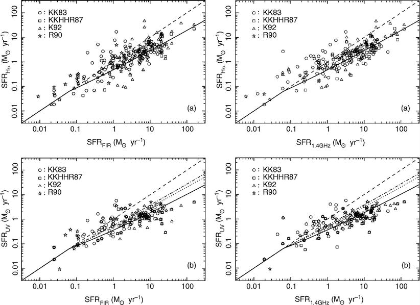
Fig. 9.54
Correlations of the star formation rates in
a sample of galaxies, as derived from observation in different
wavebands. In all four diagrams, the dashed line marks the identity relation
SFR i = SFR
j ; as is
clearly seen, using the Hα
luminosity and UV radiation as star-formation indicators seems to
underestimate the SFR. Since radiation may be absorbed by dust at
these wavelengths, and also since the amount of warm dust probably
depends on the SFR itself, this effect can be corrected for, as
shown by the solid curves
in the four panels. Source: A.M. Hopkins et al. 2001,
Toward a Resolution of the
Discrepancy between Different Estimators of Star Formation
Rate, AJ 122, 288, p. 291, Figs. 2, 3. ©AAS. Reproduced with
permission
9.6.2 Redshift dependence of the star formation: The Madau diagram
The density of star formation, ρ SFR, is defined as the
mass of newly formed stars per year per unit (comoving) volume,
typically measured in  .
Therefore, ρ SFR
as a function of redshift specifies how many stars have formed at
any time. By means of the star-formation density we can examine the
question, for instance, of whether the formation of stars began
only at relatively low redshifts, or whether the conditions in the
early Universe were such that stars formed efficiently even at very
early times.
.
Therefore, ρ SFR
as a function of redshift specifies how many stars have formed at
any time. By means of the star-formation density we can examine the
question, for instance, of whether the formation of stars began
only at relatively low redshifts, or whether the conditions in the
early Universe were such that stars formed efficiently even at very
early times.Investigations of the SFR in galaxies, by means
of the above indicators, and source counts of such star-forming
galaxies, allow us to determine ρ SFR. The plot of these
results (Fig. 9.55) is sometimes called “Madau diagram”. In
about 1996, Piero Madau and his colleagues accomplished, for the
first time, an estimate of the SFR at high redshifts from
Lyman-break galaxies in the Hubble Deep Field North. For these
early results, the intrinsic extinction was neglected. In order to
correct for this extinction, the progress in FIR and sub-millimeter
astronomy was extremely important, as we saw in Sect. 9.3.3.
There is a strong increase in ρ SFR from the current epoch
to z = 1 by about a factor
10, a further slight increase towards z ∼ 2, and a decrease at redshifts
beyond z ∼ 3. These results
have more recently been confirmed by investigations with the
Spitzer and Herschel satellites, observing a large sample of
galaxies at FIR wavelengths. Whereas the star-formation rate
density at low redshifts is dominated by galaxies which are not
very prominent at FIR wavelength, this changes drastically for
redshifts z ≳ 0. 7, above
which most of the star-formation activity is hidden from the
optical view by dust.8 The increasing importance of
dust-obscured star formation is concluded from the very strong
redshift evolution of the infrared luminosity function of galaxies
shown in Fig. 9.43, and the corresponding evolution of the
infrared luminosity density (Fig. 9.44).
Integrating the star-formation density over
cosmic time, one obtains the stellar mass density as a function of
redshift, shown in Fig. 9.56. From this we conclude that most stars in
the present-day Universe were already formed at high redshift: star
formation at earlier epochs was considerably more active than it is
today. Although the redshift-integrated star-formation rate and the
mass density of stars determined from galaxy surveys slightly
deviate from each other, the degree of agreement is quite
satisfactory if one recalls the assumptions that are involved in
the determination of the two quantities: besides the uncertainties
discussed above in the determination of the star-formation rate, we
need to mention in particular the shape of the IMF of the newly
formed stars for the determination of the stellar mass density. In
fact, Fig. 9.56 shows that we have observed the formation
of essentially the complete current stellar density.
The difference between the observed stellar mass
density and the one predicted from Fig. 9.55 is largest at high
redshifts, which may be due to the uncertainties with which
ρ SFR is
determined at high redshifts. With the more recent very deep fields
observed with HST, the unobscured star-formation rate can be
estimated at larger redshifts, based on the luminosity function of
Lyman-break galaxies (Fig. 9.41). The result is shown in Fig. 9.57, which shows a steep
decline of ρ SFR
towards higher redshift.9 Hence, the bottom line is that there
was an epoch in the Universe, between redshifts ∼ 1 and ∼ 4, where
the star-formation activity was largest. This epoch coincides with
the period in our Universe where the QSO activity was
highest—indicating that the built-up of the supermassive black hole
mass in the Universe happened in parallel to the formation of the
stellar population. The close correlation between SMBH mass and
properties of the stellar population discussed in
Sect. 3.8.3 may thus find a first
explanation in this parallel evolution.
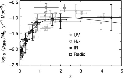
Fig. 9.55
The comoving star-formation density
ρ SFR as a
function of redshift, where the different symbols denote different
indicators used for the determination of the star-formation rate.
This plot shows the history of star formation in the Universe.
Clearly visible is the strong decline for z < 1; towards higher redshifts,
ρ SFR seems to
remain approximately constant. The curve is an empirical fit to the data.
Source: E.F. Bell 2004, Galaxy Assembly, astro-ph/0408023,
Fig. 1. Reproduced by permission of the author

Fig. 9.56
Redshift evolution of the mass density in
stars, as measured from various galaxy surveys. The solid curve specifies the integrated
star-formation density from Fig. 9.55. Source: E.F. Bell 2004, Galaxy Assembly, astro-ph/0408023,
Fig. 2. Reproduced by permission of the author
Different modes of
star formation. Whereas most of the star formation in the
local Universe occurs in spiral and irregular galaxies at a modest
rate (so-called quiescent star formation), the star-formation
activity at higher redshifts was dominated by bursts of star
formation, as evidenced in the sub-mm galaxies and in LBGs. At a
redshift z ∼ 1, the latter
has apparently ceased to dominate, yielding the strong decline of
the star-formation rate density from then until today. This
behavior may be expected if bursts of star formation are associated
with the merging of galaxies ; the merger rate declines strongly
with time in models of the Universe dominated by a cosmological
constant. This transition may also be responsible for the onset of
the Hubble sequence of galaxy morphologies around z ∼ 1.
The starburst-AGN
connection. The just-mentioned coincidence of the ‘QSO
epoch’ with the peak of the star-formation activity can either have
a statistical origin, or there can be a connection
object-by-object, in the sense that QSO are hosted in galaxies with
active star formation. For physical reasons, one would in fact
expect such a direct connection, since both processes, star
formation and AGN fueling, need a gas supply.

Fig. 9.57
Based on deep HST imaging in the optical
and near-infrared, the star-formation density ρ SFR and stellar mass
density was estimated to higher redshifts. Left panel: Blue points (and right
axis) show the UV-luminosity density as a function of redshift,
which is proportional to the unobscured star-formation rate
density. The red points
(left axis) show the star-formation rate density where a correction
for obscured star formation is included; this correction is assumed
to be negligible for z ≳ 7.
The contribution from galaxies with M UV ≤ −18 in AB magnitudes
are added up for these estimates. Black and green points are estimates of
ρ SFR and the
UV-luminosity density for z ≤ 3. The points at z ∼ 10 is based on LBG candidates
detected behind lensing clusters of the CLASH survey. Right panel: The stellar mass density
as a function of redshift. For high redshifts, ρ ∗ decreases approximately
 , as indicated by the
dashed grey curve. Source:
Left: R.J. Bouwens et
al. 2012, A Census of
Star-Forming Galaxies in the z ∼ 9 − 10 Universe based on
HST+Spitzer Observations Over 19 CLASH clusters: Three Candidate z
∼ 9 − 10 Galaxies and Improved Constraints on the Star Formation
Rate Density at z ∼ 9. 2, arXiv:1211.2230, Fig. 10.
Right: V. Gonzalez et
al. 2011, Evolution of Galaxy
Stellar Mass Functions, Mass Densities, and Mass-to-light Ratios
from z ∼ 7 to z ∼ 4,
ApJ 735, L34, p. 6, Fig. 4. ©AAS. Reproduced with permission
, as indicated by the
dashed grey curve. Source:
Left: R.J. Bouwens et
al. 2012, A Census of
Star-Forming Galaxies in the z ∼ 9 − 10 Universe based on
HST+Spitzer Observations Over 19 CLASH clusters: Three Candidate z
∼ 9 − 10 Galaxies and Improved Constraints on the Star Formation
Rate Density at z ∼ 9. 2, arXiv:1211.2230, Fig. 10.
Right: V. Gonzalez et
al. 2011, Evolution of Galaxy
Stellar Mass Functions, Mass Densities, and Mass-to-light Ratios
from z ∼ 7 to z ∼ 4,
ApJ 735, L34, p. 6, Fig. 4. ©AAS. Reproduced with permissionIndeed, in a large fraction of QSOs, clear signs
of star-formation activity are found, in some cases at a level
where the QSO host galaxy appears as a ULIRG. Conversely, in many
of the low-redshift star-forming galaxies, signs of the presence of
an AGN are seen. Furthermore, a direct connection between these two
processes in a given galaxy does not necessarily have to be
observable: it is conceivable that a fresh supply of gas (say, from
a major merging of two galaxies) first leads to a strong
star-formation activity, and that the accretion onto the central
black hole occurs with some delay—or in reverse order.
Statistical studies based on the MIR and FIR
emission properties of X-ray selected AGNs suggest that for
low-luminosity AGNs, there is no correlation between AGN luminosity
and star-formation rate. However, at high AGN luminosity, such a
correlation is indeed found, providing a strong hint for the
connection between the built-up of the black hole mass and the
stellar population in individual sources.
9.6.3 Summary: High-redshift galaxies
In this chapter, we have considered various
aspects of galaxies in the high-redshift Universe. Our discussion
of this very quickly evolving field is not complete, but
concentrates on some of the central issues. Before we move to
another class of high-redshift sources, we want to summarize some
of the points mentioned before:
-
High-redshift galaxies can be selected by a number of different methods, the most famous one being the Lyman-break technique, other multi-(optical and NIR) band selections, narrow-band imaging targeting highly-redshifted Lyα emitters, mid-infrared selection, and far-infrared/(sub-)millimeter selection. Spectroscopic confirmation of these candidates can be quite challenging, in particular for very dusty galaxies which can be very faint in the optical and NIR spectral regime, and when the source redshift approaches ∼ 7, so that the Lyα line is shifted out of the optical window.
-
As is true for other situations as well, the properties of the galaxy sample obtained depend on the selection method. A comparison of different samples can therefore be difficult, and must proceed with great care. Lyman-break galaxies at z ∼ 3 have a stellar mass smaller by a factor ∼ 10 than sub-millimeter galaxies, but larger masses than Lyman-alpha emitters.
-
The galaxy population at high redshift is distinctly different from that in the current Universe. Most galaxies at z > 2 do not fit into Hubble’s morphological classification, but show irregular light distributions. The star-formation activity in the Universe was far more intense in the past than it is now. At z ∼ 2. 5, some 10 % of all stars had been formed, and about 50 % of the stars in the local Universe were in place at z ∼ 1. Correspondingly, the average star-formation rate of distant galaxies is much higher than that of local galaxies. This is reflected in the strong evolution of the galaxy luminosity function in wavebands which strongly respond to the star-formation activity—most notably at mid-IR, far-IR and (sub-)millimeter wavelengths. Similarly, the star-formation rate density is a strongly evolving function of redshift, with a more than tenfold increase between today and z ∼ 1, an extended period of redshift lasting to z ∼ 3 or 4, where the star-formation density stays at a high rate, before declining towards even higher redshifts.
-
On the other hand, even at z ∼ 2. 5, about half of the most massive galaxies are quiescent, that is, they must have formed their large stellar population at even higher redshifts. From the evolution of the luminosity function with redshift, it appears that the most massive galaxies formed most of their stars early on, and lower-mass galaxies finish most of their evolution at lower redshifts. This trend has been termed ‘downsizing’ in the literature.
-
The mean metallicity of galaxies evolves with redshift. At a fixed stellar mass, the metallicity of galaxies at z = 2 is about smaller by a factor ∼ 2 than today, and a further factor of ∼ 2 decrease is found at z ∼ 3. 5. On the other hand, the gas of high-redshift QSOs seems to be fairly enriched with metals, approaching Solar metallicity. The dust content of galaxies appears to decrease towards the highest available redshifts, with dust-poor and almost dust-free QSOs detected at z ∼ 6.
-
Except for the CMB, which is a relic of the Big Bang, the radiation in the Universe can be understood by the cumulative emission from active and inactive galaxies in the Universe; there are no clear signs of additional source of the extragalactic background radiation. A large fraction of the background radiation can be resolved into individual sources.
9.7 Gamma-ray bursts
Discovery and
phenomenology. In 1967, surveillance satellites for the
monitoring of nuclear test ban treaties discovered γ-flashes similar to those that are
expected from nuclear explosions. However, these satellites found
that the flashes were not emitted from Earth but from the opposite
direction—hence, these γ-flashes must be a phenomenon of
cosmic origin. Since the satellite missions were classified, the
results were not published until 1973. The sources were named
gamma-ray bursts
(GRB).
The flashes are of very different duration, from
a few milliseconds up to ∼ 100 s, and they differ strongly in their
respective light curves (see Fig. 9.58). They are observed
in an energy range from ∼ 100 keV up to several MeV, sometimes to
even higher energies.
The nature of GRBs had been completely unclear
initially, because the accuracy with which the location of the
bursts was determined by the satellites was totally insufficient to
allow an identification of any corresponding optical or X-ray
source. The angular resolution of these γ-detectors was many degrees (for some,
a 2π solid angle). A more
precise position was determined from the time of arrival of the
bursts at the location of several satellites, but the error box was
still too large to search for counterparts of the source in other
spectral ranges.
Early
models. The model favored for a long time included accretion
phenomena on neutron stars in our Galaxy. If their distance was
D ∼ 100 pc, the
corresponding luminosity would be about L ∼ 1038 erg∕s, thus about
the Eddington luminosity of a neutron star. Furthermore,
indications of absorption lines in GRBs at about 40 and 80 keV were
found, which were interpreted as cyclotron absorption corresponding
to a magnetic field of ∼ 1012 Gauss—again, a
characteristic value for the magnetic field of neutron stars.
Hence, most researchers before the early 1990s thought that GRBs
occur in our immediate Galactic neighborhood.

Fig. 9.58
Gamma-ray light curves of various gamma-ray
bursts; the different time-scales on the x-axis should be particularly noted.
All these light curves appear to be very dissimilar. Credit:
J.T. Bonnell, GLAST Science Support Center, NASA/Goddard Space
Flight Center, Greenbelt, Maryland, USA
The extragalactic
origin of GRBs. A fundamental breakthrough was then achieved
with the BATSE experiment on-board the Compton Gamma Ray
Observatory, which detected GRBs at a rate of about one per day
over a period of 9 years. The statistics of these GRBs shows that
GRBs are isotropically distributed on the sky (see
Fig. 9.59),
and that the flux distribution N( > S) clearly deviates, at low fluxes,
from the S
−1. 5-law. These two results meant an end to those
models that had linked GRBs to neutron stars in our Milky Way,
which becomes clear from the following argument.
Neutron stars are concentrated towards the disk
of the Galaxy, hence the distribution of GRBs should feature a
clear anisotropy—except for the case that the typical distance of
the sources is very small ( ≲ 100 pc), much smaller than the
scale-height of the disk. In the latter case, the distribution
might possibly be isotropic, but the flux distribution would
necessarily have to follow the Euclidean law , as expected for a
homogeneous distribution of sources, which was discussed in
Sect. 4.1.2. Because this is clearly not
the case, a different distribution of sources is required, hence
also a different kind of source.
, as expected for a
homogeneous distribution of sources, which was discussed in
Sect. 4.1.2. Because this is clearly not
the case, a different distribution of sources is required, hence
also a different kind of source.
, as expected for a
homogeneous distribution of sources, which was discussed in
Sect. 4.1.2. Because this is clearly not
the case, a different distribution of sources is required, hence
also a different kind of source.The only way to obtain an isotropic distribution
for sources which are typically more distant than the disk
scale-height is to assume sources at distances considerably larger
than the distance to the Virgo cluster, hence D ≫ 20 Mpc; otherwise, one would
observe an overdensity in this direction. In addition, the
deviation from the  -law means that we
observe sources up to the edge of the distribution (or, more
precisely, that the curvature of spacetime, or the cosmic evolution
of the source population, induces deviations from the Euclidean
counts), so that the typical distance of GRBs should correspond to
an appreciable redshift. This implies that the total energy in a
burst has to be E ∼ 1051 to
1054 erg. This energy corresponds to the rest mass
Mc 2 of a star.
The major part of this energy is emitted within ∼ 1 s, so that GRBs
are, during this short time-span, more luminous than all other
γ-sources in the Universe
put together.
-law means that we
observe sources up to the edge of the distribution (or, more
precisely, that the curvature of spacetime, or the cosmic evolution
of the source population, induces deviations from the Euclidean
counts), so that the typical distance of GRBs should correspond to
an appreciable redshift. This implies that the total energy in a
burst has to be E ∼ 1051 to
1054 erg. This energy corresponds to the rest mass
Mc 2 of a star.
The major part of this energy is emitted within ∼ 1 s, so that GRBs
are, during this short time-span, more luminous than all other
γ-sources in the Universe
put together.
Fig. 9.59
Distribution of gamma-ray bursts on the
sphere as observed by BATSE, an instrument on-board the
CGRO-satellite, during the about 9 year mission; in total, 2704
GRBs are displayed. The color of
the symbols represents the observed strength (fluence, or
energy per unit area) of the bursts. One can see that the
distribution on the sky is isotropic to a high degree. Credit:
G. Fishman et al., BATSE, CGRO, NASA
We note that the estimated energy of a GRB
assumes that the relation between observed flux and luminosity is
given by L = 4π D L 2
S. This relation is valid
only for source which emit isotropically. We have seen that this
assumption breaks down for some classes of objects, for example
blazars, for which relativistic beaming plays a major role.
Identification and
afterglows. In February 1997, the first identification of a
GRB in another wavelength band was accomplished by the X-ray
satellite Beppo-SAX. Within a few hours of the burst, Beppo-SAX
observed the field within the GRB error box and discovered a
transient source, by which the positional uncertainty was decreased
to a few arcminutes. In optical observations of this field, a
transient source was then detected as well, very accurately
defining the position of this GRB. The optical source was
identified with a faint galaxy. Optical spectroscopy of the source
revealed the presence of absorption features at redshift
z = 0. 835; hence, this GRB
must have a redshift equal or larger than this. For the first time,
the extragalactic nature of GRBs was established directly. In fast
progression, other GRBs could be identified with a transient
optical source, and some of them show transient radiation also at
other wavelengths, from the radio band up to X-rays. The
lower-energy radiation of a GRB after the actual burst in
gamma-rays is called an afterglow.
With the launch of the SWIFT satellite in
November 2004, the observations of GRBs entered a new phase. This
satellite is equipped with three instruments: a wide-field
gamma-ray telescope to discover the GRBs, an X-ray telescope, and
an optical/UV telescope. Within a few seconds of the discovery of a
GRB, the satellite targets the location of the burst, so that it
can be observed by the latter two telescopes, obtaining an accurate
position. This information is then immediately transmitted to the
ground, where other telescopes can follow the afterglow emission
and obtain spectroscopic information. In its first 8 years of
operation, SWIFT discovered some 700 GRBs, of which ∼ 200 have
their redshift determined. The afterglow could be studied in a much
more homogeneous way than before. The prompt γ-ray emission carries about the same
amount of total energy as the afterglow emission in the X-ray
regime, whereas the total energy of the optical afterglow is
smaller by a factor ∼ 100.
Relativistic
motion. A GRB detected in May 1997 showed an afterglow also
at radio frequencies. In the first ∼ 20 days, its radio light curve
varied erratically, before it settled into a smoother behavior,
with flux declining in time. The flux fluctuations in the initial
light curve were interpreted as being due to scintillation in the
inhomogeneous interstellar medium, very much like the scintillation
in the Earth atmosphere.10 The end of the fluctuating period
is then interpreted as being due to the growing size of the
emitting source: Just like planets are not scintillating due to
their large angular size on the sky, interstellar scintillations
are observable only for sufficiently small sources. Hence, these
observations provided a clear evidence for an expanding source
responsible for the radio afterglow, as well as an estimate of the
source size at the end of the scintillation period, of order a few
light-weeks. Hence, the expansion velocity of the source must be of
order of the speed of light.
There is another independent argument for the
presence of relativistic motion in GRBs. The short time-scale of
the γ-ray emission,
together with its large flux, implies that the density of
γ-ray photons in the source
must be extremely high. In such a situation, the γ-rays are subject to a large opacity
for  -pair production—in
other word, the γ-rays
cannot escape from the source region, but are efficiently
transformed into pairs. To escape this conclusion, Doppler boosting
needs to be employed (cf. Sect. 5.5.2). Allowing for relativistic
velocities along our line-of-sight, the radiation density in the
source declines significantly. Furthermore, the estimated source
size, based on variability argument, increases if Doppler boosting
is at work. With a Lorentz factor of the bulk motion of
-pair production—in
other word, the γ-rays
cannot escape from the source region, but are efficiently
transformed into pairs. To escape this conclusion, Doppler boosting
needs to be employed (cf. Sect. 5.5.2). Allowing for relativistic
velocities along our line-of-sight, the radiation density in the
source declines significantly. Furthermore, the estimated source
size, based on variability argument, increases if Doppler boosting
is at work. With a Lorentz factor of the bulk motion of
![$$\gamma = [1 - (v/c)^{2}]^{-1/2} \sim 10^{2}$$](A129044_2_En_9_Chapter_IEq24.gif) or
larger, the pair-production opacity constraints can be avoided, and
source sizes of order 1013 cm can be accomplished.
or
larger, the pair-production opacity constraints can be avoided, and
source sizes of order 1013 cm can be accomplished.
-pair production—in
other word, the γ-rays
cannot escape from the source region, but are efficiently
transformed into pairs. To escape this conclusion, Doppler boosting
needs to be employed (cf. Sect. 5.5.2). Allowing for relativistic
velocities along our line-of-sight, the radiation density in the
source declines significantly. Furthermore, the estimated source
size, based on variability argument, increases if Doppler boosting
is at work. With a Lorentz factor of the bulk motion of
or
larger, the pair-production opacity constraints can be avoided, and
source sizes of order 1013 cm can be accomplished.Fireball
model. Hence, GRBs are associated with a relativistic
phenomenon, but the question of their nature still remained
unanswered. One model of GRBs quite accurately describes their
emission characteristics, including the afterglow. In this fireball
model, the radiation is released in the relativistic outflow of
electron-positron pairs with a Lorentz-factor of γ ≥ 100. This radiation is not
isotropic, but most likely concentrated in a rather narrow beam,
resembling the jets in AGNs. In order to form such collimated
outflows, one needs a strong energy source, and presumably strong
rotation whose rotation axis defines the preferred directions into
which the jets flow. To collimate the jets, the presence of
magnetic fields are probably also required.
Short vs.
long-duration bursts. GRBs can be broadly classified into
short- and long-duration bursts, with a division at a duration of
t burst ∼ 2 s.
The spectral index of the short-duration bursts is considerably
harder at γ-ray energies
than that of long-duration bursts. Until 2005, only afterglows from
long-duration bursts had been discovered. Long-duration bursts
typically occur in galaxies at high redshift, with a mean of
z ∼ 2. 5. Also GRBs with
very high redshift were discovered, with at least three having
redshifts z > 6. One GRB
redshift of z = 8. 2 has
been spectroscopically obtained, and there are indications that an
even higher-redshift burst was observed. In one case, an optical
burst was discovered about 30 seconds after the GRB, with the
fantastic brightness of V ∼ 9, at a redshift of z = 1. 6. For a short period of time,
this source was apparently more luminous than any quasar in the
Universe. In March 2008, a GRB at z = 0. 937 occurred which has a peak
optical brightness of m = 5. 7—i.e., this source was visible
for a very short period to the naked eye (it is not known, though,
whether anyone peeked at the right position of the sky at that
moment). Thus, during or shortly after the burst at high energies,
GRBs can also be very
bright in the optical.
Counterparts of
long-duration GRBs: Hypernovae. In April 1998, the
positional error box of a GRB contained a supernova, hinting for a
possible connection. This has been verified subsequently, by
finding that the light-curve of some optical afterglows were
described by the sum of a declining power law in time plus the
light-curve of a luminous supernova. For a GRB in March 2003, the
presence of a supernova in the spectrum of the optical afterglow
was identified, proving the direct connection between SNe and GRBs.
Since most of the GRBs are located at high redshifts, the
corresponding SN cannot be identified for them, but for more nearby
long-duration bursts, the association is clearly established.
Long-duration GRBs are located in star-forming
regions of galaxies, and their redshift distribution is similar to
that of the star-formation rate density in the Universe.11 This observation yields
a close connection of the GRB phenomenon to star formation, and
thus the associated supernovae are due to young massive stars. Not
every core-collapse SN yields a GRB, though. The current picture is
that GRBs are produced in the core-collapse process of very massive
stars, giving rise to extraordinarily energetic explosions,
so-called hypernovae. The combination of stellar rotation and an
internal magnetic field can form a highly relativistic
bi-directional outflow after the collapse event, when the stellar
material falls onto the newly formed compact remnant, a black hole.
Even if the emission is highly anisotropic, as expected from the
fireball model, the corresponding energy released by the hypernovae
is very large.
Counterparts of
short-duration GRBs. SWIFT has allowed the identification of
afterglow emission from short-duration GRBs. In contrast to the
long-duration bursts, some of these seem to be associated with
elliptical galaxies; this essentially precludes any association
with (core-collapse) supernova explosions. In fact, for one of
these short burst, very sensitive limits on the optical brightness
explicitly rules out any contribution from a supernova explosion.
Furthermore, the host galaxies of short bursts are at substantially
lower redshift, z ≲ 0. 5.
Given that both kinds of GRBs have about the same observed flux (or
energy), this implies that short-duration bursts are less energetic
than long-duration ones, by approximately two orders of magnitude.
All of these facts clearly indicate that short- and long-duration
GRBs are due to different populations of sources. The lower
energies of short bursts and their occurrence in early-type
galaxies with old stellar populations are consistent with them
being due to the merging of compact objects, either two neutron
stars, or a neutron star and a black hole.
Footnotes
1
Readers not familiar with the optical/near-IR
filter system may find it useful to consult Sect. A.4.2 in the
Appendix at this point. We will also follow the usual practice and
write R = 22 instead of
R = 22 mag in the
following.
2
Whereas the symbols for redshift and the
z-band magnitudes are
identical, we trust that no confusion will arise by that, as the
meaning will always be clear by the context.
3
Note that a factor of 5 in magnification
corresponds to a factor 25 in the exposure time required for
spectroscopy. This factor of 25 makes the difference between an
observation that is feasible and one that is not. Whereas the
proposal for a spectroscopic observation of 3 h exposure time at an
8-m telescope may be successful, a similar proposal of 75 h would
be hopelessly doomed to failure.
4
At the time of writing, ∼ 90 QSOs with
z > 5. 7 and known, of
which ∼ 40 have z > 6. 0; those were found from
several wide-field imaging surveys, including SDSS, the CFHT quasar
survey, the UKIRT Infrared Deep Sky Survey (UKIDSS), and
Pan-STARRS.
5
The accuracy with which the position of a compact
source can be determined is approximately given by the ratio of the
FWHM and the signal-to-noise ratio with which this source is
observed.
6
The reason for this bias is the very different
K-correction in the sub-mm and radio regimes, due to the very
different slopes of the spectral energy distribution in these two
regimes, as can be seen in Fig. 9.30: Whereas the flux in the sum-mm regime
increases as a source is moved to higher redshifts, its radio flux
decreases strongly, thus biasing against the detection of
high-z SMGs in the
radio.
7
There a few TeV blazars at higher redshift, but
as we discussed in Sect. 5.2.6, the featureless spectrum of
most blazars renders the determination of a secure redshift
sometimes uncertain.
8
We recall that the roughly equal energy in the
optical and FIR extragalactic background radiation shows that about
half of the cosmic star formation occurs in dust-obscured
regions.
9
The derivation of the star-formation rate as a
function of redshift is largely drawn from galaxy surveys which are
based on color selection, such as LBGs, EROs and sub-mm galaxies.
The possibility cannot be excluded that additional populations of
galaxies which are luminous but do not satisfy any of these
photometric selection criteria are present at high redshift. Such
galaxies can be searched for by spectroscopic surveys, extending to
very faint magnitude limits. This opportunity now arises as several
of the 10-m class telescopes are now equipped with high multiplex
spectrographs which can thus take spectra of many objects at the
same time. One of them is VIMOS at the VLT, another is DEIMOS on
Keck. With both instruments, extensive spectroscopic surveys are
being carried out on flux-limited samples of galaxies. Among the
first results of these surveys is the finding that there are indeed
more bright galaxies at redshift z ∼ 3 than previously found, by about a
factor of 2, leading to a corresponding correction of the
star-formation rate at high redshifts. In a color-color diagram,
these galaxies are preferentially located just outside the
selection box for LBGs (see Fig. 9.4). Given that this selection box was chosen
such as to yield a high reliability of the selected candidates, it
is not very surprising that a non-negligible fraction of galaxies
lying outside, but near to it are galaxies at high redshift with
similar properties.
10
Recall that atmospheric scintillations are due to
a space and time dependent refractive index of the air. For
propagating radio waves, the same is true, except that the
refractive index here is determined by the electron density of the
ionized plasma in the ISM.
11
Indeed, it seems that the distribution of GRBs
extends further out in redshift than that of the star formation
density. This observational fact is most likely related to the
finding that GRBs are found in host galaxies with small
metallicity. It is possible that the metal enrichment of galaxies
suppresses GRBs at later redshifts. The connection to the
metallicity may have its origin on a possible metallicity-dependent
star formation, i.e., allowing for higher-mass stars from
metal-poor gas.