SENSORS AND THEIR MEASUREMENTS FOR OCEAN MONITORING
This chapter discusses sensors for ocean monitoring and their measuring parameters. Sometimes satellites are called sensors, as well as the sensors they carry. It discusses the sensors, scanners, weather sensing, SAR sensors, marine observation sensors (MOS), ocean color monitoring sensor (OCM) and micro-sensors for ocean acidification monitoring. It also discusses the measurement of ocean parameters, such as ocean color, sediment monitoring, surface currents, surface wind, wave height, wind speed, sea surface temperature, upwelling, sampling, wave energy, and ocean floor. It also describes spatial resolution, pixel size, scale, spectral/radiometric resolution, temporal resolution, sensor design, sensor selection, and research on ocean phenomena.
2.1INTRODUCTION TO SENSORS
A passive remote sensing system records the energy naturally radiated or reflected from an object. An active remote sensing system supplies its own source of energy, which is directed at the object to measure the returned energy [Figure 2.1]. Flash photography is active remote sensing, in contrast to available light photography, which is passive. Another common form of active remote sensing is radar, which provides its own source of electromagnetic energy in the microwave region. Airborne laser scanning is a relatively new form of active remote sensing, operating in the visible and near infrared wavelength bands.

For a sensor to collect and record energy reflected or emitted from a target or surface, it must reside on a stable platform removed from the target or surface being observed. Platforms for remote sensors may be situated on the ground, on an aircraft or balloon (or some other platform within the Earth’s atmosphere), or on a spacecraft or satellite outside of the Earth’s atmosphere. Ground-based sensors are often used to record detailed information about the surface which is compared with information collected from aircraft or satellite sensors. In some cases, this can be used to better characterize the target that is being imaged by these other sensors, making it possible to better understand the information in the imagery. Sensors may be placed on a ladder, scaffolding, tall building, cherry-picker, crane, etc. Aerial platforms are primarily stable wing aircraft, although helicopters are occasionally used. Aircraft are often used to collect very detailed images and facilitate the collection of data over virtually any portion of the Earth’s surface at any time. In space, remote sensing is sometimes conducted from the space shuttle or, more commonly, from satellites. Satellites are objects which revolve around another object—in this case, the Earth. For example, the moon is a natural satellite, whereas manmade satellites include those platforms launched for remote sensing, communication, and telemetry (location and navigation) purposes. Because of their orbits, satellites permit repetitive coverage of the Earth’s surface on a continuing basis. Cost is often a significant factor in choosing among the various platform options.
Since the early 1960s, numerous satellite sensors have been launched into orbit to observe and monitor the Earth and its environment. Most early satellite sensors acquired data for meteorological purposes. The advent of earth resources satellite sensors (those with a primary objective of mapping and monitoring land cover) occurred when the first LANDSAT satellite was launched in July 1972. Currently, more than a dozen orbiting satellites of various types provide data crucial to improving our knowledge of the Earth’s atmosphere, oceans, ice and snow, and land. The path followed by a satellite is referred to as its orbit. Satellite orbits are matched to the capability and objective of the sensor(s) they carry. Orbit selection can vary in terms of altitude (their height above the Earth’s surface) and their orientation and rotation relative to the Earth. Satellites at very high altitudes, which view the same portion of the Earth’s surface at all times, have geostationary orbits [Figure 2.2]. These geostationary satellites, at altitudes of approximately 36,000 km, revolve at speeds which match the rotation of the Earth, so they seem stationary relative to the Earth’s surface. This allows the satellites to observe and collect information continuously over specific areas. Weather and communications satellites commonly have these types of orbits. Due to their high altitude, some geostationary weather satellites can monitor weather and cloud patterns covering an entire hemisphere of the Earth.
Many remote sensing platforms are designed to follow an orbit (basically north-south) which, in conjunction with the Earth’s rotation (west-east), allows them to cover most of the Earth’s surface over a certain period. These are near-polar orbits, so named for the inclination of the orbit relative to a line running between the North and South Poles. Many of these satellite orbits are also sun-synchronous such that they cover each area of the world at a constant local time of day called local sun time. At any given latitude, the position of the sun in the sky as the satellite passes overhead will be the same within the same season. This ensures consistent illumination conditions when acquiring images in a specific season over successive years, or over a particular area over a series of days. This is an important factor for monitoring changes between images as they do not have to be corrected for different illumination conditions.

FIGURE 2.2 Satellite orbits.
Most of the remote sensing satellite platforms today are in near-polar orbits, which means that the satellite travels northwards on one side of the Earth and then toward the southern pole on the second half of its orbit. These are called ascending and descending passes, respectively. If the orbit is also sun-synchronous, the ascending pass is most likely on the shadowed side of the Earth while the descending pass is on the sunlit side. Sensors recording reflected solar energy only image the surface on a descending pass, when solar illumination is available.
Active sensors which provide their own illumination or passive sensors that record emitted (e.g., thermal) radiation can also image the surface on ascending passes. As a satellite revolves around the Earth, the sensor “sees” a certain portion of the Earth’s surface. The area imaged on the surface is referred to as the swath [Figure 2.3]. Imaging swaths for space-borne sensors generally vary between tens and hundreds of kilometers wide. As the satellite orbits the Earth from pole to pole, its east-west position wouldn’t change if the Earth didn’t rotate. However, as seen from the Earth, it seems that the satellite is shifting westward because the Earth is rotating (from west to east) beneath it. This apparent movement allows the satellite swath to cover a new area with each consecutive pass. The satellite’s orbit and the rotation of the Earth work together to allow complete coverage of the Earth’s surface, after it has completed one complete cycle of orbits.

FIGURE 2.3 Ascending and descending pass and swath.
If we start with any randomly selected pass in a satellite’s orbit, an orbit cycle will be completed when the satellite retraces its path, passing over the same point on the Earth’s surface directly below the satellite (called the nadir point) for a second time. The exact length of time of the orbital cycle will vary with each satellite. The interval of time required for the satellite to complete its orbit cycle is not the same as the revisit period. Using steerable sensors, a satellite-borne instrument can view an area (off-nadir) before and after the orbit passes over a target, thus making the “revisit” time less than the orbit cycle time. The revisit period is an important consideration for many monitoring applications, especially when frequent imaging is required (for example, to monitor the spread of an oil spill, or the extent of flooding). In near-polar orbits, areas at high latitudes will be imaged more frequently than the equatorial zone due to the increasing overlap in adjacent swaths as the orbit paths come closer together near the poles.
2.2SCANNER SENSOR SYSTEMS
Electro-optical and spectral imaging scanners produce digital images with the use of detectors that measure the brightness of reflected electromagnetic energy. Scanners consist of one or more sensor detectors depending on type of sensor system used. One type of scanner is called a whiskbroom scanner, also referred to as across-track scanners (e.g., on a LANDSAT satellite). It uses rotating mirrors to scan the landscape below from side to side perpendicular to the direction of the sensor platform, like a whiskbroom. The width of the sweep is referred to as the sensor swath. The rotating mirrors redirect the reflected light to a point where a single or just a few sensor detectors are grouped together. Whiskbroom scanners with their moving mirrors tend to be large and complex to build. The moving mirrors create spatial distortions that must be corrected with preprocessing by the data provider before image data is delivered to the user. An advantage of whiskbroom scanners is that they have fewer sensor detectors to keep calibrated as compared to other types of sensors.
Another type of scanner, which does not use rotating mirrors, is the pushbroom scanner, also referred to as an along-track scanner (e.g., on SPOT). The sensor detectors in a pushbroom scanner are lined up in a row called a linear array. Instead of sweeping from side to side as the sensor system moves forward, the 1-dimensional sensor array captures the entire scan line at once, like a pushbroom would. Step stare scanners contain 2-dimensional arrays in rows and columns for each band. Pushbroom scanners are lighter, smaller, and less complex because of fewer moving parts than whiskbroom scanners, and they have better radiometric and spatial resolution. A major disadvantage of pushbroom scanners is the calibration required for the large number of detectors that make up the sensor system [Figure 2.4].

FIGURE 2.4 Scanners.
2.2.1Spatial Resolution, Pixel Size, and Scale
For some remote sensing instruments, the distance between the target being imaged and the platform plays a large role in determining the detail of information obtained and the total area imaged by the sensor. Sensors on platforms far away from their targets typically view a larger area but cannot provide great detail. Compare what an astronaut onboard the Space Shuttle sees of the Earth to what you can see from an airplane. The astronaut might see your whole province or country in one glance, but couldn’t distinguish individual houses. Flying over a city or town, you would be able to see individual buildings and cars, but you would be viewing a much smaller area than the astronaut. There is a similar difference between satellite images and air photos. The detail discernible in an image is dependent on the spatial resolution of the sensor and refers to the size of the smallest possible feature that can be detected.
Spatial resolution of passive sensors depends primarily on their instantaneous field of view (IFOV in Figure 2.5). The IFOV is the angular cone of visibility of the sensor (A) and determines the area on the Earth’s surface that is “seen” from a given altitude at one particular moment in time (B). The size of the area viewed is determined by multiplying the IFOV by the distance from the ground to the sensor (C). This area on the ground is called the resolution cell and determines a sensor’s maximum spatial resolution. For a homogeneous feature to be detected, its size generally has to be equal to or larger than the resolution cell. If the feature is smaller than this, it may not be detectable as the average brightness of all features in that resolution cell will be recorded. However, smaller features may sometimes be detectable if their reflectance dominates within an articular resolution cell, allowing subpixel or resolution cell detection.
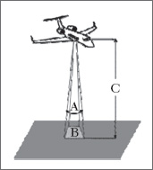
FIGURE 2.5 Instantaneous field of view (IFOV).
Most remote sensing images are composed of a matrix of picture elements, or pixels, which are the smallest units of an image. Image pixels are normally square and represent a certain area on an image. It is important to distinguish between pixel size and spatial resolution—they are not interchangeable. If a sensor has a spatial resolution of 20 meters and an image from that sensor is displayed at full resolution, each pixel represents an area of 20 meters 20 meters on the ground. In this case the pixel size and resolution are the same. However, it is possible to display an image with a pixel size different than the resolution. Many posters of satellite images of the Earth have their pixels averaged to represent larger areas, although the original spatial resolution of the sensor that collected the imagery remains the same.
A photograph can be represented and displayed in a digital format [Figure 2.6] by subdividing the image into small, equal-sized and -shaped areas, called picture elements or pixels, and representing the brightness of each area with a numeric value or digital number.

FIGURE 2.6 Satellite images.
Images where only large features are visible are said to have coarse or low resolution. In fine or high resolution images, small objects can be detected. Military sensors for example, are designed to view as much detail as possible, and therefore have very fine resolution. Commercial satellites provide imagery with resolutions varying from a few meters to several kilometers. Generally speaking, the finer the resolution, the less total ground area can be seen. The ratio of distance on an image or map, to actual ground distance is referred to as scale. If you had a map with a scale of 1:100,000, an object of 1 cm length on the map would actually be an object 100,000 cm (1 km) long on the ground. Maps or images with small map-to-ground ratios are referred to as small scale (e.g., 1:100,000), and those with larger ratios (e.g., 1:5,000) are called large scale.
2.2.2Spectral/Radiometric Resolution
Spectral characteristics: While the arrangement of pixels describes the spatial structure of an image, the radiometric characteristics describe the actual information content in an image. Every time an image is acquired on film or by a sensor, its sensitivity to the magnitude of the electromagnetic energy determines the radiometric resolution. The radiometric resolution of an imaging system describes its ability to discriminate very slight differences in energy. The finer the radiometric resolution of a sensor, the more sensitive it is to detecting small differences in reflected or emitted energy.
Digital resolution is the number of bits comprising each digital sample. Imagery data are represented by positive digital numbers which vary from 0 to (one less than) a selected power of 2. This range corresponds to the number of bits used for coding numbers in binary format. Each bit records an exponent of power 2 (e.g., 1 bit = 21 = 2). The maximum number of brightness levels available depends on the number of bits used in representing the energy recorded. Thus, if a sensor used 8 bits to record the data, there would be 28 = 256 digital values available, ranging from 0 to 255—also called the dynamic range of the system. However, if only 4 bits were used, then only 24 = 16 values ranging from 0 to 15 would be available. Thus, the radiometric resolution would be much less. Image data are generally displayed in a range of grey tones, with black representing a digital number of 0 and white representing the maximum value (for example, 255 in 8-bit data). By comparing a 2-bit image with an 8-bit image, we can see that there is a large difference in the level of detail discernible depending on their radiometric resolutions.
The range of energy values expected from a system must fit within the range of values possible of the data format type, and yet the value must represent accurately the energy value of the signal relative to others. The cost of more bits per data point is longer acquisition times, the need for larger storage capacity, and longer processing time. Any signal outside the range is clipped and thus unrecoverable. On the other hand, if the dynamic range of the signal is widened too much to allow the recording of extremely high or low energy values, the true variability within the signal will be lost.
Many remote sensing systems record energy over several separate wavelength ranges at various spectral resolutions. These are referred to as multi-spectral sensors. Advanced multi-spectral sensors, called hyper-spectral sensors, detect hundreds of very narrow spectral bands throughout the visible, near-infrared, and mid-infrared portions of the electromagnetic spectrum. Their very high spectral resolution facilitates fine discrimination between different targets based on their spectral response in each of the narrow bands. There are four general parameters that describe the capability of a spectrometer: 1) spectral range, 2) spectral bandwidth, 3) spectral sampling, and 4) signal-to-noise ratio (S/N).
Spectral range: Spectral range is important to cover enough diagnostic spectral absorption to solve a problem. There are general spectral ranges that are in common use, each to first order controlled by detector technology: a) ultraviolet (UV): 0.001 to 0.4 μm, b) visible: 0.4 to 0.7 μm, c) near-infrared (NIR): 0.7 to 3.0 μm, d) the mid-infrared (MIR): 3.0 to 30 μm, and d) the far infrared (FIR): 30 μm to 1 mm. The 0.4 to 1.0-μm wavelength range is sometimes referred to in the remote sensing literature as the VNIR (visible-near-infrared) and the 1.0 to 2.5-μm range is sometimes referred to as the SWIR (short-wave infrared).
Spectral bandwidth: Spectral bandwidth is the width of an individual spectral channel in the spectrometer. The narrower the spectral bandwidth, the narrower the absorption feature the spectrometer will accurately measure, if enough adjacent spectral samples are obtained. All the spectra are sampled at half Nyquist (critical sampling) except the near infrared mapping spectrometer (NIMS), which is at Nyquist sampling (named after H. Nyquist, who in his work published in 1928 stated that there must be at least two samplings per wavelength of the highest frequency in order to appropriately sample the waveform). Note, however, that the fine details of the absorption features are lost at the ~25 nm bandpass of NIMS. The visual and infrared mapping spectrometer (VIMS) and NIMS systems measure out to 5 μm and thus can see absorption bands not obtainable by the other systems.
Spectral sampling: Spectral sampling is the distance in wavelength between the spectral bandpass profiles for each channel in the spectrometer as a function of wavelength. The Nyquist theorem states that the maximum information is obtained by sampling at one-half the full width at half maximum (FWHM).
Signal-to-noise ratio: Finally, a spectrometer must measure the spectrum with enough precision to record details in the spectrum. The signal-to-noise ratio (S/N) required to solve a problem will depend on the strength of the spectral features under study. The S/N is dependent on the detector sensitivity, the spectral bandwidth, and intensity of the light reflected or emitted from the surface being measured. A few spectral features are quite strong and a S/N of only about 10 will be adequate to identify them, while others are weak, and a S/N of several hundred (and higher) are often needed.
2.2.3Temporal Resolution
In addition to spatial, spectral, and radiometric resolution, the concept of temporal resolution is also important to consider in a remote sensing system. The revisit period of a satellite sensor is usually several days. Therefore, the absolute temporal resolution of a remote sensing system to image the exact same area at the same viewing angle a second time is equal to this period. However, the actual temporal resolution of a sensor depends on a variety of factors, including the satellite/sensor capabilities, the swath overlap, and latitude.
The ability to collect imagery of the same area of the Earth’s surface at different periods of time is one of the most important elements for applying remote sensing data. Spectral characteristics of features may change over time and these changes can be detected by collecting and comparing multi-temporal imagery. For example, during the growing season, most species of vegetation are in a continual state of change and our ability to monitor those subtle changes using remote sensing is dependent on when and how frequently we collect imagery. By imaging on a continuing basis at different times we can monitor the changes that take place on the Earth’s surface, whether they are naturally occurring (such as changes in natural vegetation cover or flooding) or induced by humans.
The time factor in imaging is important when:
 Persistent clouds offer limited
clear views of the Earth’s surface (often in the tropics)
Persistent clouds offer limited
clear views of the Earth’s surface (often in the tropics)
Short-lived phenomena (floods,
oil slicks, etc.) need to be imaged
Multi-temporal comparisons are
required
The changing appearance of a
feature over time can be used to distinguish it from near-similar
features
2.2.4Sensor Design and Selection
Each remote sensing mission has unique requirements for spatial, spectral, radiometric, and temporal resolution. A number of practical considerations also arise in the design process, including system development and operational costs; the technical maturity of a particular design; and power, weight, volume, and data rate requirements. Because it is extremely expensive, or perhaps impossible, to gather data with all the characteristics a user might want, the selection of sensors or satellite subsystems for a mission involving several tasks generally involves compromises. Sensor performance may be measured by spatial and spectral resolution, geographical coverage, and repeat frequency. For example, sensors with very high spatial resolution are typically limited in geographical coverage. A video camera is one example of an instrument that employs an electro-optical sensor. The sun’s angle with respect to the surface varies somewhat throughout the year, depending on the sun’s apparent position with respect to the equator.
2.3WEATHER SATELLITES/SENSORS
Weather monitoring and forecasting was one of the first civilian applications of satellite remote sensing. Today, several countries operate weather or meteorological satellites to monitor weather conditions around the globe. These satellites use sensors which have fairly coarse spatial resolution (when compared to systems for observing land) and provide large areal coverage. Their temporal resolutions are generally quite high, providing frequent observations of the Earth’s surface, atmospheric moisture, and cloud cover, which allows for near-continuous monitoring of global weather conditions, and hence forecasting. These weather satellites carry sensors related to weather monitoring.
As India’s first domestic dedicated Earth resources satellite program, the IRS series provides continuous coverage of the country. An indigenous ground system network handles data reception, data processing, and data dissemination. India’s National Natural Resources Management System (NNRMS) uses IRS data to support a large number of applications projects.
India has orbited IRS satellites which carry two payloads employing linear imaging selfscanning sensors (LISS). The IRS-series have a 22-day repeat cycle. The LISS-I imaging sensor system consists of a camera operating in four spectral bands, compatible with the output from LANDSAT-series Thematic Mapper and SPOT HRV instruments. The LISS-IIA and B comprise two cameras operating in visible and near-infrared wavelengths with a ground resolution of 36.5 meters and swath width of 74.25 km. As part of the National Remote Sensing Agency’s international services, IRS data are available to all countries within the coverage zone of the Indian ground station located at Hyderabad. These countries can purchase the raw/processed data directly from NRSA Data Centre. India is designing sensors with resolutions of about 20 meters in multi-spectral bands and better than 10 meters in the panchromatic band. System designers intend to include a short-wave infrared band with spatial resolution of 70 meters. The system will also include a wide field sensor (WiFS) with 180 meter spatial resolution and larger swath of about 770 km for monitoring vegetation.
Operational uses of ocean satellites: The development and operation of SeaSat demonstrated the utility of continuous ocean observations, not only for scientific use, but also for those concerned with navigating the world’s oceans and exploiting ocean resources. Its success convinced many that an operational ocean remote sensing satellite would provide significant benefits. The SAR, the scatterometer, and the altimeter all gathered data of considerable utility. Knowledge of currents, wind speeds, wave heights, and general wave conditions at a variety of ocean locations is crucial for enhancing the safety of ships at sea and for ocean platforms. Such data could also decrease costs by allowing ship owners to predict the shortest, safest sea routes.
SeaSat carried five major instruments—an altimeter, a microwave radiometer, a scatterometer, a visible and infrared radiometer, and synthetic aperture radar (SAR). Scientists used data from these instruments to measure the amplitude and direction of surface winds, absolute and relative surface temperature, the status of ocean features such as islands, shoals, and currents, and the extent and structure of sea ice. Data from the SeaWifs instrument aboard the privately developed SeaStar satellite will provide ocean color information, which could have considerable operational use.
Observations of sea ice: Because sea ice covers about 13% of the world’s oceans, it has a marked effect on weather and climate. Thus, measurements of its thickness, extent, and composition help scientists understand and predict changes in weather and climate. Until satellite measurements were available, the difficulties of tracking these characteristics were a major impediment to understanding the behavior of sea ice, especially its seasonal and yearly variations. The AVHRR visible and infrared sensors aboard have been used to follow the large-scale variations in the Arctic and Antarctic ice packs. Because they can “see through” clouds, synthetic aperture radar instruments are particularly useful in tracking the development and movement of ice packs, which pose threats to shipping, and in finding routes through the ice.
2.4SYNTHETIC APERTURE RADAR SENSORS
Synthetic aperture radar (SAR) image data provide information different from that of optical sensors operating in the visible and infrared regions of the electromagnetic spectrum. SAR data consist of high-resolution reflected returns of radar-frequency energy from terrain that has been illuminated by a directed beam of pulses generated by the sensor. The radar returns from the terrain are mainly determined by the physical characteristics of the surface features (such as surface roughness, geometric structure, and orientation), the electrical characteristics (dielectric constant, moisture content, and conductivity), and the radar frequency of the sensor. By supplying its own source of illumination, the SAR sensor can acquire data day or night without regard to cloud cover.
2.5MARINE OBSERVATION SATELLITES (MOS) SENSORS
The Earth’s oceans cover more than two-thirds of the Earth’s surface and play an important role in the global climate system. They also contain an abundance of living organisms and natural resources which are susceptible to pollution and other man-induced hazards. The Nimbus-7 satellite, launched in 1978, carried the first sensor, the coastal zone color scanner (CZCS), specifically intended for monitoring the Earth’s oceans and water bodies. The primary objective of this sensor was to observe ocean color and temperature, particularly in coastal zones, with sufficient spatial and spectral resolution to detect pollutants in the upper levels of the ocean and to determine the nature of materials suspended in the water column. The Nimbus satellite was placed in a sun-synchronous, near-polar orbit at an altitude of 955 km. Equator crossing times were local noon for ascending passes and local midnight for descending passes. The repeat cycle of the satellite allowed for global coverage every six days, or every 83 orbits. The CZCS sensor consisted of six spectral bands in the visible, near-IR, and thermal portions of the spectrum each collecting data at a spatial resolution of 825 m at nadir over a 1566 km swath width. The accompanying table outlines the spectral ranges of each band and the primary parameter measured by each.
TABLE 2.1 CZCS Spectral Bands
As can be seen from the Table 2.1, the first four bands of the CZCS sensor are very narrow. They were optimized to allow detailed discrimination of differences in water reflectance due to phytoplankton concentrations [Figure 2.7] and other suspended particulates in the water. In addition to detecting surface vegetation on the water, band 5 was used to discriminate water from land prior to processing the other bands of information. The CZCS sensor ceased operation in 1986.

FIGURE 2.7 CZCS sensor image.
Marine observation satellite (MOS): The first Marine Observation Satellite carries three different sensors: a four-channel multispectral electronic self-scanning radiometer (MESSR), a four-channel visible and thermal infrared radiometer (VTIR), and a two-channel microwave scanning radiometer (MSR), in the microwave portion of the spectrum. The characteristics of the two sensors in the visible/infrared are described in Table 2.2.
The MESSR bands are thus useful for land applications in addition to observations of marine environments. The MOS systems orbit at altitudes around 900 km and have revisit periods of 17 days.

Sea-viewing wide-field-of view sensor (SeaWiFS): The SeaWiFS (sea-viewing wide-field-of view sensor) on board the SeaStar spacecraft is an advanced sensor designed for ocean monitoring. It consists of eight spectral bands of very narrow wavelength tailored for very specific detection and monitoring of various ocean phenomena including: ocean primary production and phytoplankton processes, ocean influences on climate processes (heat storage and aerosol formation), and monitoring of the cycles of carbon, sulfur, and nitrogen. The orbit altitude is 705 km with a local equatorial crossing time of 12 PM. Two combinations of spatial resolution and swath width are available for each band: a higher resolution mode of 1.1 km (at nadir) over a swath of 2,800 km, and a lower resolution mode of 4.5 km (at nadir) over a swath of 1,500 km. These ocean-observing satellite systems are important for global and regional scale monitoring of ocean pollution and health and assist scientists in understanding the influence and impact of the oceans on the global climate system.
Oceansat: Oceansat-2 is an Indian satellite designed to provide the ocean color monitor (OCM) instrument for users. It will also enhance the potential of applications in other areas. The main objectives of OceanSat are to study surface winds and ocean surface strata, observation of chlorophyll concentrations, monitoring of phytoplankton blooms, and study of atmospheric aerosols and suspended sediments in the water. (This is explained in detail in Appendix A: Indian Satellites for Ocean Monitoring.)
2.6MICRO SENSORS FOR MONITORING OCEAN ACIDIFICATION
New technology that will measure pH levels in seawater with a cost-effective micro sensor for long-term monitoring of ocean acidification has been developed. Ocean acidification is occurring due to rising levels of atmospheric carbon dioxide (CO2), which is absorbed by the oceans. When it dissolves in seawater, CO2 forms a mild acid, which is decreasing ocean pH globally and could impact marine ecosystems. As well as monitoring global change, the sensors can be used to measure more localized human impact. The micro sensors could be deployed to detect leakages from carbon capture and storage sites—whereby CO2 is artificially removed from the atmosphere and stored in subsea reservoirs—by measuring any proximal fluctuations in pH. The oil industry is also interested in this technology for monitoring seawater acidity around drilling sites.
The sensor works on the principles of litmus paper color changes depending on the acidity of the solution. The microfluidic chip within the sensor has great advantages because it is robust, small, reasonably cheap to produce, and uses small amounts of reagents—which is really key for in situ deployment where it may be collecting data out at sea for long periods of time. The sensor uses a dye which changes color with pH. The dye is added to the sample, then the color is measured using an LED light source and a device called a “spectrometer.” The microfluidic element simply describes the component needed to mix the seawater sample with the dye and the cell to measure the color. The microfluidic chip used in the pH micro sensor with dimensions: 13 × 8 cm is shown in Figure 2.8.

FIGURE 2.8 (a) pH micro sensor and (b) VULCANO buoy with atmospheric and communication sensors.
The VULCANO buoy with atmospheric and communication sensors is shown in Figure 2.8b. The increase in the production and emission of anthropogenic CO2 and its absorption by the oceans leads to a reduction in oceanic pH, a process referred to as ocean acidification, which affects many other physicochemical processes. Atmospheric CO2 is expected to continue its increase, and consequently the chemical changes will likely continue well into the future, affecting the ocean biogeochemical cycling. To characterize the ocean’s chemical and ecosystem-related changes, examination of CO2 system parameters over a wide range of temporal and spatial scales is necessary. Shipboard analyses in oceanic time series conducted during irregular ocean expeditions, which lasted between a fortnight and a month, have provided most of our understanding of recent trends in the oceanic CO2 system. However, our ability to make frequent autonomous measurements over a broad range of spatial scales would greatly augment the current suite of open-ocean and coastal observations.
The carbon dioxide system in natural waters is defined by the measurement of two or more carbonate parameters: pH, carbon dioxide fugacity (fCO2), total alkalinity (TA), and total dissolved inorganic carbon (DIC). The sensors for pH, pCO2, DIC, and TA of seawater have been developed based in spectrophotometric techniques that in most cases require accurate dye additions and consideration of the effects of aging. A new family of rugged and extremely stable spectrophotometric pH sensors for both lab-based research and buoy monitoring, specifically designed for unattended operation independently of dye and aging effects in surface waters, is also developed.
2.7MEASUREMENTS OF OCEAN MONITORING PARAMETERS
Satellite sensors have been developed to operate either in the optical infrared part of the electromagnetic spectrum (λ-0.4–12 μm) or in the microwave part (λ-0.3–30 μm). These sensors, either from an aircraft or satellite, have measured the basic sea surface properties to useful accuracies. These properties of sea are color, temperature, slope/height and roughness etc. At present all ocean features—physical, chemical, biological, or geological—must produce a surface signature in one of those parameters if they are to be monitored from space; that is, for example, chlorophyll concentrations must affect ocean color (and possibly temperature), bottom topography must be reflected in sea surface shapes (and possibly roughness), surface waves must modulate small-scale surface roughness patterns, and so on.
Ocean color data is a vital resource for a wide variety of operational forecasting and oceanographic research, earth sciences, and related applications. Some of them are
Mapping of chlorophyll
concentrations
Measurement of inherent optical
properties such as absorption and backscatter
Determination of phytoplankton
physiology, phenology, and functional groups
Studies of ocean carbon fixation
and cycling
Monitoring of ecosystem changes
resulting from climate change
Fisheries management
Mapping of coral reefs, sea grass
beds, and kelp forests
Mapping of shallow-water
bathymetry and bottom type for military operations
Monitoring of water quality for
recreation
Ocean color is the measurement of spectral distribution of radiance (or reflectance) upwelling from the ocean in the visible regime. Measurements of ocean color from space can provide quantitative maps of near-surface phytoplankton pigment concentration as well as identifying pollutants spilled into the sea by effluent discharges. The spectral composition of the radiation above the sea (that is, its color) is determined by the composition of solar irradiance plus the optical properties of the water column—in particular, the absorption, scattering, and to a lesser degree the fluorescence. The optical properties of the water column are, in turn, determined by those of pure sea water plus the concentrations of suspended and dissolved materials within it particulate organic matter (phytoplankton and its byproducts), inorganic suspended particles, and dissolved organic decay products of mainly terrestrial origin (yellow substance).
However, in the shorter term, fisheries research can be assisted enormously by a more precise knowledge of the elements in the food chain—larval recruitment, zooplankton production, and the patchiness of plankton. In this regard color (and temperature) information derived from orbiting satellites is particularly useful in tropical and subtropical regions. The requirement to monitor the spread of pollutants may be stronger in some areas than others. In closed or semi-enclosed seas such as the North Sea or Mediterranean, the indiscriminate dumping of waste products into the sea has become a major source of concern and in many respects the ocean color signal can be detected and traced from satellites. Color imagery has also been successfully exploited in dynamical studies of the physics of shallow sea processes.

FIGURE 2.9 This MODIS image of blue water in the Caribbean Sea looks blue because the sunlight is scattered by the water molecules. Near the Bahama Islands, the lighter aqua colors are shallow water where the sunlight is reflecting off of the sand and reefs near the surface.
The “color” of the ocean is determined by the interactions of incident light with substances or particles present in the water. White light from the sun is made up of a combination of colors, which are broken apart by water droplets in a “rainbow” spectrum. When light hits the water surface, the different colors are absorbed, transmitted, scattered, or reflected in differing intensities by water molecules and other optically active constituents in the upper layer of the ocean.
If there are any particles suspended in the water, they will increase the scattering of light. For example, microscopic marine algae, called phytoplankton, have the capacity to absorb light in the blue and red region of the spectrum owing to specific pigments like chlorophyll. Accordingly, as the concentration of phytoplankton increases in the water, the color of the water shifts toward the green part of the spectrum. Fine mineral particles like sediment absorb light in the blue part of the spectrum, causing the water to turn brownish in case of massive sediment load.
The basic principle behind the remote sensing of ocean color from space is, the more phytoplankton in the water, the greener it is, and the less phytoplankton, the bluer it is. There are other substances that may be found dissolved in the water that can also absorb light. These substances are referred as colored dissolved organic matter (CDOM).
Ocean color sensors: Active remote sensing is a signal of known characteristics and sent from the sensor platform—an aircraft or satellite—to the ocean, and the return signal is then detected after a time delay determined by the distance from the platform to the ocean and by the speed of light. One example of active remote sensing at visible wavelengths is the use of laser-induced fluorescence to detect chlorophyll, yellow matter, or pollutants. In laser fluorosensing, a pulse of UV light is sent to the ocean surface, and the spectral character and strength of the induced fluorescence at UV and visible wavelengths gives information about the location, type, and concentration of fluorescing substances in the water body. Another example of active remote sensing is LIDAR bathymetry. This refers to the use of pulsed lasers to send a beam of short duration, typically about a nanosecond, toward the ocean. The laser light reflected from the sea surface and then slightly later from the bottom is used to deduce the bottom depth. The depth is simply 0.5(c/n) Δt, where c is the speed of light in vacuum, n is the water index of refraction, Δt is the time between the arrival of the surface-reflected light and the light reflected by the bottom, and the 0.5 accounts for the light traveling from the surface to the bottom and back to the surface.
Passive remote sensing simply observes the light that is naturally emitted or reflected by the water body. The nighttime detection of bioluminescence from aircraft is an example of the use of emitted light at visible wavelengths. The most common example of passive remote sensing is the use of sunlight that has been backscattered within the water and returned to the sensor. This light can be used to deduce the concentrations of chlorophyll, CDOM, or mineral particles within the near-surface water; the bottom depth and type in shallow waters; and other ecosystem information such as net primary production, phytoplankton functional groups, or phytoplankton physiological state.
Passive ocean color remote sensing from satellites began with the coastal zone color scanner (CZCS), which was launched in 1978. CZCS was a multi-spectral sensor, meaning that it had only a few wavelength bands with bandwidths of 10 nm or more. After the phenomenal success of that “proof of principle” sensor, numerous other multi-spectral sensors have been developed and launched. Those later sensors generally had a few more bands with narrower bandwidths. Thus, the sea-viewing wide field-of-view sensor (SeaWiFS) added a band near 412 nm to improve the detection of CDOM. The near-IR bands are used for atmospheric correction. There is today much interest in the use of hyperspectral sensors, which typically have 100 or more bands with nominal bandwidths of 5 nm or less. Figure 2.10 shows the wavelength bands for a few representative sensors. The MODIS (MODerate resolution Imaging Spectro radiometer) sensor has additional bands in the 400–900 nm range, which are used for detection of clouds, aerosols, and atmospheric water vapor. The bands shown are the ones used for remote sensing of water bodies. The compact airborne hyperspectral imager (CASI) is a commercially available hyperspectral sensor that is widely used in airborne remote sensing of coastal waters. It has 228 slightly overlapping bands, each with a nominal 1.9 nm bandwidth and covering the 400–1000 nm range. CASI users often select a subset of these bands as needed for an application. LIDAR bathymetry systems typically use either 488 nm in “blue” water or 532 nm in “green” water. Those wavelengths can be obtained from high-power lasers and give close to optimum water penetration for the respective water types.

FIGURE 2.10 Wavelength bands used by various ocean color remote sensors.
Although remote sensing usually obtains information for one spatial point at a time, most applications combine measurements from many points to build up an image, i.e., a 2D spatial map of the ocean displaying the desired information at a given time. Imagery acquired at different times then gives temporal information. Satellite systems typically have spatial resolution (the size of one image pixel at the ocean surface) of 250 meters to 1 km. Those systems are useful for regional to global scale studies. Airborne systems can have resolutions as small as 1 meter, as required for applications such as mapping coral reefs.
Passive ocean-color remote sensing is conceptually simple. Sunlight, whose spectral properties are known, enters the water body. The spectral character of the sunlight is then altered, depending on the absorption and scattering properties of the water body, which of course depend on the types and concentrations of the various constituents of the water body. Part of the altered sunlight eventually makes its way back out of the water and is detected by the sensor on board an aircraft or satellite. If we know how different substances alter sunlight, for example by wavelength-dependent absorption, scattering, or fluorescence, then we can deduce from the altered sunlight what substances must have been present in the water and in what concentrations. This process of working backwards from the sensor to the ocean is an inverse problem that is fraught with difficulties. Nevertheless, these difficulties can be overcome, and ocean color remote sensing has completely revolutionized our understanding of the oceans at local to global spatial scales and daily to decadal temporal scales.
Ocean color radiometry: Ocean color radiometry is a technology, and a discipline of research, concerning the study of the interaction between the visible electromagnetic radiation coming from the sun and aquatic environments. In general, the term is used in the context of remote-sensing observations, often made from Earth-orbiting satellites. Using sensitive radiometers, one can measure carefully the wide array of colors emerging out of the ocean. These measurements can be used to infer important information such as phytoplankton biomass or concentrations of other living and nonliving material [Figure 2.11] that modify the characteristics of the incoming radiation.
Start time of the remote sensing of color: Remote sensing of ocean color from space began in 1978 with the successful launch of NASA’s coastal zone color scanner (CZCS). Ten years passed before other sources of ocean-color data became available with the launch of other sensors, and in particular the sea-viewing wide field-of-view sensor (SeaWiFS) in 1997 on board the NASA SeaStar satellite. Subsequent sensors have included NASA’s moderate-resolution imaging spectroradiometer (MODIS) on board the Aqua and Tearra satellites and ESA’s medium resolution imaging spectrometer (MERIS) on board its environmental satellite Envisat. Several new ocean-color sensors have recently been launched, including the Indian ocean color monitor (OCM-2) on board ISRO’s Oceansat-2 satellite, the Korean geostationary ocean color imager (GOCI), which is the first ocean color sensor to be launched on a geostationary satellite, and the visible infrared imager radiometer suite (VIIRS) aboard NASA’s Suomi NPP. More ocean color sensors are planned over the next decade by various space agencies. Table 2.4 gives information about the sensing of ocean color sensors launched by various agencies and Table 2.5 gives information about scheduled color sensors.


How satellites “see” ocean color: Satellite instruments or sensors “see” variations in the color of the ocean by detecting different wavelengths or bands of reflected light. The colors are recorded as numerical values that can be downloaded and converted back into images. Scientists can then compare the color in satellite images at specific times and locations to actual measurements of chlorophyll or other suspended matter in samples of ocean water collected at the same time and location. The comparison, called ground truthing, enables scientists to develop mathematical formulas or algorithms for analyzing the same parameters in other satellite images. This technique has enabled scientists to track the timing and spread of offshore phytoplankton blooms around the oceans, which has helped explain the timing and success of year classes—fish in a stock that hatched in the same year.
Satellite imagery and ground truthing: Collecting ground truth data is essential to interpreting what satellite instruments “see” in the ocean. Ground truthing involves comparing pixels on a satellite image with direct observations and measurements on the ground or, in this case, the ocean. This enables scientists to verify what they are seeing in the image and to convert the colors to tangible quantities, such as biomass of plankton or sediment concentration. Satellite and ground truth data must be collected at the same time and location.
It is easier to interpret offshore satellite images because the only thing that changes the color of the ocean, other than the water itself, is the presence of phytoplankton. Interpreting near shore satellite imagery is more complicated because in addition to phytoplankton, other suspended matter including sediment and colored dissolved organic matter (CDOM) from terrestrial matter such as decomposing leaves can change the ocean color and we don’t necessarily know which factor has a more significant effect. Since the main source of CDOM is from the land, concentrations vary with river outflow and rainfall. This means that an algorithm for the near shore that is valid for today may not be valid tomorrow and we will probably have to develop separate ones for different seasons, conditions, and locations.
Coastal zone color scanner: The CZCS measured ocean color in four discrete bands with a further low sensitivity band designed for coast and cloud identification. A further band in the infrared operated intermittently. The four color bands are shown in Table 2.6.
TABLE 2.6 IR Band for Ocean Color Monitoring
To understand the link between the color of the sea and the concentration of suspended matter within its surface layer, models of radiative transfer were constructed from a study of the spectral characteristics of a number of substances. Much of the approach was necessarily empirical. The total radiance observed at the sensor can effectively be divided into two components:
1.Water-leaving radiance, which is that part of the signal that has penetrated the sea surface and been reflected back, times the diffuse transmission between the sea surface and the sensor, and
2.Radiance that has not penetrated the sea surface but has been reflected or scattered from other sources into the sensor.
Whereas the effects of the ocean form part of the first, atmospheric effects dominate the second and make up the unwanted noise. The basic task of processing the CZCS record is to identify and remove this noise and then, from the water leaving part of the signal, to make the best estimate of phytoplankton pigment concentrations. Much effort has gone into the development of the best processing algorithms. Although the CZCS included reference signals for calibration, it became apparent at a comparatively early stage of the mission that the blue channel was losing sensitivity. The largest effort has been directed to correcting for atmospheric effects which have two main components: radiance resulting from molecular scattering (Raleigh), and scattering due to aerosols (Mie scattering) [also see Figure 10.1].
2.7.2Sediment Monitoring Methods
Sediment lies at the bottom of the ocean floor; it is made from many items, including:
Tiny particles of rock, sand, silt, and clay
Marine snow (clumps of living and
dead microscopic organisms, faecal pellets, and dust)
Materials vented out from the
Earth’s surface
Over time the sediment forms layer upon layer building up a record of the ocean floor at that moment. Scientists examine these layers to find out about the past. For example, the size of particles shows how close to the shore the ocean floor used to be, because large particles sink faster and therefore nearer to land.
Rock samples are collected because they can tell about:
What the rocks are made of
How the rock was formed
Mineralization—minerals can be an
important resource
The mantle—the layer underneath
the Earth’s crust
Earth’s evolution—how tectonic
plates used to be arranged
Future geohazards—earthquakes,
volcanoes, tsunamis
The goal of sediment monitoring is to quantify changes in sedimentation and soil characteristics that relate the changes in elevation, vegetation, and invertebrates. The rate of sediment accretion or erosion is a determining factor of tidal wetland sustainability with sea level rise and a primary driver of habitat evolution over time. Accretion rates vary spatially due to many factors including elevation, vegetation type and productivity, distance to channels, wave climate, and salinity dynamics. Elevation of the mud flat and the associated inundation frequency and duration are critical to understanding the potential vegetation community that will colonize post-restoration actions. In the context of climate change, long-term adaptability and persistence of tidal marsh depends in part on sediment sources, quantities, and distribution patterns. Basin scale restoration and enhancement projects, including the blocking of large naturally eroding bluffs, are projected to significantly reduce historical sediment delivery rates. In contrast, changes in the flow regime (e.g., dike removal) and in storm frequency and intensity may increase sediment delivery. Multiple methods are used to measure sedimentation in tidal marshes and should be chosen based on restoration and monitoring objectives and site-specific considerations.
The following methods can be used for repeated measures of sedimentation at localized spots over time.
1.Sediment pins
Description: Poles installed within a study site. Height of pole is measured through time to show sediment gain or loss.
Benefits: Inexpensive, easy to install and measure underwater or on land.
Limitations: Sedimentation rates limited to where pin is installed, cm resolution.
2.Sediment plates
Description: In areas of soft sediment, a hard plate is placed below the sediment surface. Measure the sediment accumulation on top of plate.
Benefits: Easy, inexpensive, possible to measure accumulation and erosion, reduces error of rod penetrating into soft sediments, mm resolution, can be used to calculate sediment volume.
Limitations: Plates can be undercut due to hydrologic scour.
3.Marker horizons
Description: A thick marker layer (usually white in color, i.e., feldspar clay) placed on top sediment surface. Sediment cores are later taken to measure sediment accumulation. It can be paired with surface elevation tables (SET) to explain processes behind elevation increases or decreases (i.e., sedimentation, shallow subsidence, etc.).
Benefits: Easy, inexpensive, mm resolution.
Limitations: Repeated measures can deplete marker horizon layer, can be affected by invertebrate bioturbation, does not measure erosion, can be eroded/washed away (typically in unvegetated areas, in this case, use of plastic grid or sediment plate is recommended), can be difficult to measure in areas of standing water (may need to freeze sediment core using liquid nitrogen).
4.Surface elevation table (SET):
Description: Portable mechanical leveling device for measuring relative sediment elevation changes. Is often paired with marker horizon to explain processes behind elevation increases or decreases (i.e., sedimentation, shallow subsidence, etc.).
Benefits: Accurate and precise as measurements are always taken in the exact location, mm resolution.
Limitations: Expensive to install, sedimentation rates limited to where poles are installed, poles can sometimes cause erosion in unvegetated areas.
Mapping of sea floor: Geoscientists are interested in the terrain of an area: Is it flat or rocky? Are there any canyons, mountains, or volcanoes? To find out, scientists need to map the area. On dry land, satellites can be used to measure vast areas, but in water, satellite signals (microwaves) can be absorbed. The further a signal travels through water, the less likely it is to bounce back, so another method is needed to map the ocean floor. Sound waves use pressure to move through gases, liquids, and solids. In air, sound moves at around 340 meters per second but in seawater it zooms along at around 1,500 meters per second. Light cannot be used as it is absorbed by water very quickly; usually lighting no further than 30 meters. So by using sound, scientists can find out different properties about the sea floor, as shown in Table 2.7.
| Method used | Property discovered | How it’s done |
| Single-beam echo-sounder |
Bathymetry—the measurement of depth to the bottom. Can also be used to gain information about the subsurface, i.e., deep or shallow sediment. |
Measured using the time it takes for the sound to be sent and returned. |
| Multi-beam echo-sounder |
Swath bathymetry—by taking lots of depth measurements from a single place the shape of the sea bed is revealed. |
Measured using the time it takes for the sound to be sent and returned. |
| Backscatter |
Measures the reflectivity of the floor—this will show what the floor is made of, e.g., rocks, sand, mud. |
The change to the strength of the returned sound wave. |
| Sound Velocity Profilers |
Measures the speed sound moves through the water, as it varies depending on the water properties at different depths. Important to know otherwise depth calculations will be wrong. |
Measures the temperature, and sometimes the salinity, of the water to determine the speed. |
TABLE 2.7 Properties of Sea Floor for Different Methods
The ocean is maintained in a state of continual motion through a combination of solar radiation and the earth’s rotation. Currents are produced by the equilibrium established between a number of forces which include gravity, pressure gradients within the volume of the sea, the Coriolis force due to the Earth’s rotation, and frictional forces mostly due to wind. The pressure gradients within the water column are produced by differences in density at fixed depths brought about by different values of temperature and salinity. Because the earth rotates from west to east, an observer in the Northern Hemisphere would observe that a moving object was deflected to the right (that is, in a clockwise direction). In the Southern Hemisphere the deflection is to the left, while at the equator there is no deflection. The strength of the horizontal component of the Coriolis force depends on the latitude and on the speed of a moving object such as a water particle. If there were no Coriolis force acting (that is, if the earth were not in rotation) the pressure gradient would cause the water to move directly from high to low pressure. On a rotating Earth, the Coriolis force deflects the motion; the acceleration on the water will reduce to zero when the speed of the current at given latitude is fast enough to produce a Coriolis force in exact balance with the horizontal pressure gradient. In the absence of frictional forces this balance is referred to as geostrophic flow. From the simple geostrophic relationship linking current speed and latitude to the Earth’s rate of rotation and to the acceleration due to gravity, the surface slope is easily calculated. Surface slopes produced by currents are measured against a reference equipotential mean sea level referred to as the geoid. Over the surface of the Earth, variations in the gravity field cause the geoid itself to undulate with respect to a reference ellipsoid by about 200 meters. (The minimum is found in the Indian Ocean just south of Sri Lanka while the maximum is relatively close in the Eastern Pacific off Borneo).
A method that has been used to compute patterns of sea level changes is to calculate a mean geoid over a selected area from (say) a year’s altimeter’s observations, subtract this out—making corrections to the calculated height of the altimeter by minimizing the differences at track intersections—and record the differences [Figure 2.12]. At middle and high latitudes, the cross-track difference between the Geosat ground tracks was approximately 100 km, making the altimeter observations useful for mapping the tracks of mesoscale eddies. In areas of extremely high sea level variability, the Geosat observations were used to compute a frequency-wave number spectrum of sea level variability which identified significant eddy energy at time scales longer than 34 days and spatial scales longer than 200 km.

FIGURE 2.12 Sea level.
2.7.4Surface Wind and Waves
Ever since sailors first put to sea, efforts have been made to improve the forecasts of the conditions they may find there. Sudden storms still take their toll in terms of ships and men lost at sea. Each month sees two ships disappear without trace off the face of the globe. There are strong arguments therefore for improving the collection of reliable measurements of wind and wave conditions over the oceans. One obviously successful area of international cooperation is the meteorological global network in which nations share their observations with each other. Routine measurements of surface pressure, humidity, precipitation, wind velocity, temperature, and other parameters form the basis of the weather charts issued up to four times daily around the globe. Ships play their own part in reporting conditions at sea. It remains true, however, that their observations are unevenly distributed over large tracts of open ocean, especially in the Southern Hemisphere where comparatively few are reported. It is clear that satellites will play a primary role in helping to achieve its ultimate potential. In general terms ocean waves are the result of winds blowing over the surface for a certain time (duration) and over a certain area (fetch).
The primary elements of good forecasting are:
1.accurate wind estimates over the relevant duration and fetch
2.an understanding of how winds generate waves
3.an understanding of how waves are generated, propagated, transformed, and dissipated along their route

FIGURE 2.13 Surface winds during Hurricane Ivan estimated from QuikScat scatterometer measurements.
2.7.5Wave Height and Wind Speed
The largest forces on any offshore or coastal structure, from ships to offshore rigs to coastal defenses, generally result from surface waves, which can cause destruction and devastation, in association with forces from winds, currents, and sea level surges. Ships—even 100,000-ton carriers—routinely disappear in storms; offshore structures have been severely damaged and millions of dollars of damage have been inflicted upon breakwaters in recent years. Knowledge of ocean waves is essential for any activity connected with the seas. Forecasts of wave conditions are required for operational planning, both at specified locations and across oceans for ship routing. Estimates of wave climate, such as monthly average wave height or 50-year wave height, are needed for design purposes. Forecasts are prepared using numerical wave models with forecast winds as input and using the physics of wave growth, transmission, and decay developed in recent years, but forecasts are considerably improved if the models are initiated and updated with observations of wave height and period.
2.7.6Sea Surface Temperature
The ocean-atmosphere system is a heat engine powered by solar radiation. The average daily amount of incoming radiation decreases from the equator to the poles. Low latitudes receive relatively large amounts of radiation each year while winter darkness and the obliqueness of the sun’s rays reduce the amount of radiation received at the higher latitudes. The Earth also reemits radiation from the sun at slightly longer wavelengths, most of which is absorbed by natural greenhouse gases in the atmosphere such as carbon dioxide, water vapor, and cloud droplets. There is a net gain of radiation energy at low latitudes and a net loss at higher latitudes. But since there is no net gain of heat at low latitudes (or loss at higher latitudes) there must be a net transfer of heat to maintain a balance. This is brought about mainly through winds in the atmosphere and currents in the oceans. In the tropics, it is the oceans which contribute more to the poleward transfer of heat while the atmosphere contributes more at the higher latitudes. Across the equator, the oceans provide the mechanism for a southward net transport from the Northern to the Southern Hemisphere. The two principal components of the ocean contribution are wind-driven surface currents and density-driven (thermohaline) deep circulation. Of the total amount of energy received from the sun by the oceans, about 41% is lost to the atmosphere as long-wave radiation and about 54% as latent heat by evaporation from the sea surface. Temperature is a measure of the thermal energy possessed by the oceans and if the average temperature is to remain constant then the gains and losses must even out—that is, the heat budget must balance.
Sea surface temperature (SST) is observed at low frequencies generally in the range of 5–10 GHz. The great advantage of microwave sensors for measuring SST over the more commonly used infrared instruments is their ability to operate through cloud but this must be offset against their resolution of around 150 km, which is too coarse to study mesoscale eddies. Higher resolution would require a much larger antenna than has been flown up to now. Another constraint is contamination by land masses, and in general reliable measurements must be made in the open ocean more than 600 km from a coast. Thus, again, interesting ocean features such as boundary current and their associated eddy may not be capable of being studied with the microwave radiometer.
Measurements of ocean parameters by microwave radiometers are affected by atmospheric water vapor, clouds, and rainfall and most sensors are therefore backed up by frequencies sensitive to water in the atmosphere. This information is also of considerable importance where precise altimetry is required to measure very small changes in ocean topography. It is the role of the ocean in redistributing heat by currents and mixing which ultimately will be one of the key factors in determining whether or not there will be a net warming over the globe due to a manmade increase in greenhouse gases. Attempts to measure the oceanic heat transport directly by traditional observations have been less than successful in providing credible estimates.
This is particularly true in the Southern Hemisphere, where observations are so sparse that neither the magnitude nor even the direction of heat transport estimated directly agree with those inferred from the apparent global radiation budget. Patterns of surface temperature revealed by satellite have been used to study the flow of currents by following certain distinguishable features, shown in Figure 2.14.
In a similar way, sea surface temperature has been used to infer other variables in the upper ocean. Upwelling around the coasts of many tropical and subtropical countries carries a strong temperature signal which can be identified and studied from space-borne infrared devices. By their very nature many such areas also exhibit a strong increase in phytoplankton, as revealed in the record of the coastal zone color scanner. Thus, in some areas sea surface temperature may be used as a useful tracer of nutrient concentrations. Sea surface temperature (SST) is an important geophysical parameter, providing the boundary condition used in the estimation of heat flux at the air-sea interface. On the global scale this is important for climate modeling, study of the earth’s heat balance, and insight into atmospheric and oceanic circulation patterns. On a more local scale, SST can be used operationally to assess eddies, fronts, and upwellings for marine navigation and to track biological productivity. Satellite technology has improved upon our ability to measure SST by allowing frequent and global coverage. In the past, SST could only be measured by ships and buoys, whose ranges were limited. Figure 2.15 shows two maps illustrating this point.

Methods for determining SST from satellite remote sensing include thermal infrared and passive microwave radiometry. Interest in using satellites to measure ocean phenomena began in the 1960s. In 1978, the polarorbiting TIROS satellites began to gather data on sea surface temperatures using the AVHRR and microwave sensors. The maps of sea surface temperatures produced from these data demonstrate complex surface temperature patterns that have led to considerable speculation about the physical processes that might cause such patterns. However, it was not until NASA launched Nimbus 7 and SeaSat in 1978 that scientists were able to gather comprehensive measurements of the oceans. Nimbus-7 carried a scanning multichannel microwave radiometer (SMMR) that provided accurate measurements of sea surface temperatures. By measuring the color of the ocean surface, its coastal zone color scanner (CZCS) provided estimates of ocean biological productivity.

Thermal infrared SST measurements: Thermal infrared SST measurements have a long heritage (~20 years). They are derived from radiometric observations at wavelengths of ~3.7 μm and/or near 10 μm. Though the 3.7 μm channel is more sensitive to SST, it is primarily used only for nighttime measurements because of relatively strong reflection of solar irradiation in this wavelength region, which contaminates the retrieved radiation. Both bands are sensitive to the presence of clouds and scattering by aerosols and atmospheric water vapor. For this reason, thermal infrared measurements of SST first require atmospheric correction of the retrieved signal and can only be made for cloud-free pixels. Thus, maps of SST compiled from thermal infrared measurements are often weekly or monthly composites which allow enough time to capture cloud-free pixels over a region. Thermal infrared instruments that have been used for deriving SST include advanced very high resolution radiometer (AVHRR) on NOAA polarorbiting operational environmental satellites (POES), along-track scanning radiometer (ATSR) aboard the European remote sensing satellite (ERS-2), the geostationary operational environmental satellite (GOES) imager, and moderate resolution imaging spectroradiometer (MODIS) aboard NASA earth observing system (EOS) Terra and Aqua satellites.
Strengths: Good resolution and accuracy and long heritage (~ 20 years)
Weaknesses: Obscured by clouds and atmospheric corrections required
Passive microwave SST measurements: Due to lower signal strength of the Earth’s Planck radiation curve in the microwave region, accuracy and resolution is poorer for SST derived from passive microwave measurements compared to SST derived from thermal infrared measurements. However, the advantage gained with passive microwave is that radiation at these longer wavelengths is largely unaffected by clouds and generally easier to correct for atmospheric effects. This is well illustrated in the two SST images in Figure 2.16. Though the two images cover the same period, the thermal infrared composite (AVHRR) has lots of white patches where cloud-free pixels could not be obtained over such a short period of time.

FIGURE 2.16 Comparison between thermal infrared and passive microwave.
Phenomena which do effect passive microwave signal return, however, are wind-generated roughness at the ocean’s surface and precipitation. These can usually be corrected for, however, using multiple frequencies. SST measurements are primarily made at a channel near 7 GHz with a water vapor correction enabled by observation at 21 GHz. Other frequencies used for correction of surface roughness (including foam), precipitation, and what little effect clouds do have on microwave radiation are 11, 18, and 37 GHz. Passive microwave instruments that have been used for deriving SST include the scanning multichannel microwave radiometer (SMMR) carried on Nimbus-7 and SeaSat satellites, the tropical rainfall measuring mission (TRMM) microwave imager (TMI), and upcoming data from the advanced microwave scanning radiometer (AMSR) instrument on the NASA EOS Aqua satellite and on the Japanese advanced earth observing satellite (ADEOS II).
Strengths: Clouds are mostly transparent and relatively insensitive to atmospheric effects
Weaknesses: Poorer accuracy and resolution; sensitive to surface roughness and precipitation
Derivation of SST: Radiation emitted by a surface is the Planck emission times the surface emissivity. Since the Planck function is dependent on temperature and is well known, sea surface temperature can be estimated if the surface emissivity can be sufficiently estimated using models or regression techniques that employ independent in situ measurements. After atmospheric corrections, then, coefficients are applied to the retrieved brightness temperature signals in the derivation of SST which factor in estimations of the surface emissivity. Simple linear algorithms provide reasonably accurate SST calculations under favorable atmospheric and surface conditions, but more sophisticated higher-order computations may be required otherwise. Because of temperature gradients below the ocean’s surface, the depth at which measurements are made will significantly impact the SST. Measurements made at only a depth of one or two molecules below the ocean’s surface are considered the interface SST and cannot be realistically measured. Just below this, however, at a depth of roughly 10 μm is what is known as the skin SST. The attenuation length of thermal infrared radiation corresponds to this depth. The subskin SST is at a depth of ~1 mm and corresponds to the attenuation length of microwave radiation. Beyond this depth is what is commonly referred to as the bulk SST, near-surface SST, or SSTdepth. Figure 2.17 is an illustration of these different depths of SST, showing two different temperature gradients:
As can be discerned from Figure 2.17, the bulk SST (or SSTdepth) may vary greatly from the skin and subskin SSTs depending on the temperature gradient. The skin temperature may also vary from the subskin temperature for the same reason. Diurnal heating will cause these differences to be greatest during the afternoon and least right before dawn. Since SST measurements made from buoys and ships are usually bulk temperature measurements, temperature gradients must be taken into consideration when comparing them to SST measurements made by either thermal infrared or passive microwave remote sensing observations.
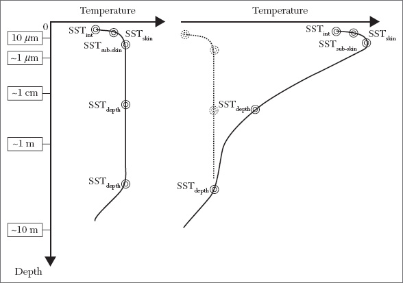
Since thermal infrared instruments measure the skin temperature and passive microwave instruments measure the subskin temperature, one must also consider differences due to evaporative cooling at the sea surface when comparing measurements derived from these methods. The difference can be as great as 1 Kelvin in combination with diurnal heating effects, and so both properties must be properly accounted for when comparing or blending thermal infrared and microwave products.
Weakness: Diurnal heating and evaporative cooling make comparison of SSTs at different depths difficult; special care must be taken to correct for their effects
Blending thermal infrared and passive microwave SST: Given the desire to combine the high accuracy and resolution of the thermal infrared SST measurements with the better temporal and spatial coverage of passive microwave SST measurements (due to cloud transparency), efforts are being made to create a blended product which combines these strengths. In the effort to combine these two kinds of SST products, careful consideration must be made to correct for differences due to diurnal heating and evaporative cooling as well as biases introduced by high wind speeds, water vapor, and other atmospheric conditions. Models are being tested for each of these considerations. Algorithms which incorporate these models still use in situ measurements, as well, to quality assure and to adjust the final product.
Strength: Helps scientists better model climate change with improved SST product
2.7.7Upwelling
Winds blowing across the ocean surface often push water away from an area. When this occurs, water rises from beneath the surface to replace the diverging surface water. This process is known as upwelling. Figure 2.18 highlights major upwelling areas along the world’s coasts. These subsurface waters are typically colder, rich in nutrients, and biologically productive. Therefore, good fishing grounds typically are found where upwelling is common. For example, the rich fishing grounds along the west coasts of Africa and South America are supported by year-round coastal upwelling.

FIGURE 2.18 Upwelling.
Properties like satellite speed, satellite ground speed, satellite period, number of orbits/day, separation of ascending track on equator, track separation, if evenly distributed for H months, and satellite precession rate determine the sampling and sampling rates. Table 2.8 describes the sampling scheme for the measurements type and notes differences between the systems.
2.7.9Wave Power
Wave power is the transport of energy by ocean surface waves, and the capture of that energy to do useful work. For example, electricity generation, water desalination, or the pumping of water (into reservoirs) is done using wave power. A machine able to exploit wave power is generally known as a wave energy converter (WEC).
2.7.10Ocean Floor
The bottom of a body of water is known as the benthic zone, regardless of how deep it occurs. In coastal waters the sea floor sits upon the continental shelf and is generally less than 200m deep. Most of the ocean floor lies upon the ocean crust and is between 4,000—6,000 meters deep. Working at such depths requires specialist tools and skills to obtain the data needed [Figure 2.19].

FIGURE 2.19 The ocean floor was mapped using an EM120 echo-sounder.
The reasons for study the benthic zone are just as varied but can include:
Understanding—exploration of
areas, learning about ecosystems and habitats
Resources—locations and
quantities of minerals, oil, gases, and food supplies
Geohazards—landslides such as the
one that caused the 2004 Tsunami, turbidity currents. It is not
safe to dump waste at sea.
Ocean sensing and the ice caps: Because the oceans cover about 70% of Earth’s surface, they make a significant contribution to Earth’s weather and climate. The oceans interact constantly with the atmosphere above them and the land and ice that bound them. Yet scientists know far too little about the details of the oceans effects on weather and climate, in part because the oceans are monitored only coarsely by ships and buoys. Improving the safety of people at sea and managing the seas vast natural resources also depend on receiving better and more timely data on ocean phenomena. Satellite remote sensing is one of the principal means of gathering data about the oceans.

TABLE 2.8 Sampling Time
2.8RESEARCH ON OCEAN PHENOMENA
To understand the behavior of the oceans and to make more accurate predictions of their future behavior, scientists need to gather data about sea temperature, surface color, wave height, the distribution of wave patterns, surface winds, surface topography, and currents. Fluctuations in ocean temperatures and currents lead to fluctuations in the atmosphere and therefore play a major part in determining weather and climate. Understanding and predicting the interactions are major goals of climatologists. The study of other ocean phenomena would enhance scientists understanding of the structure and dynamics of the ocean. For example, observations of wave conditions are important for modeling ocean dynamics. Because winds create waves, measurements of wind speed and direction over wide areas can lead to estimates of wave height and condition. Closely observing the color of the ocean surface provides a powerful means of determining ocean productivity. Variations in ocean color are determined primarily by variations in the concentrations of algae and phytoplankton, which are the basis of the marine food chain. Because these microscopic plants absorb blue and red light more readily than green light, regions of high phytoplankton concentration appear greener than those with low concentration. Because fish feed on the photoplankton, regions of high concentration indicate the possibility of greater fish population.
EXERCISES: PART A (ANSWER IN A WORD OR A SENTENCE)
1.What is passive remote sensing?
2.Give examples for active remote sensing.
3.Define “satellite orbit.”
4.What are the geostationary satellites?
5.What is the use of having remote sensing satellites in near polar orbits?
6.Define “swath.”
7.What is the other name of whiskbroom scanner?
8.Give the definition of instantaneous field of view (IFOV).
9.___________ describes the ability of the image to discriminate very slight differences in energy.
10.Define “spectral range.”
11.What is spectral bandwidth?
12.What is spectral sampling?
13.What is the importance of signal-to-noise ratio?
14.What is the significance of ocean color?
15.Define “ocean color radiometry.”
16.What is upwelling?
17.Define “wave power.”
18.What is the benthic zone?
EXERCISES: PART B (ANSWER IN A PAGE)
1.Write a note on remote sensor platforms.
2.Differentiate between passive and active remote sensing.
3.Write about scanner sensor systems.
4.Compare the whiskbroom scanner with the push broom scanner.
5.Write a note on temporal resolution.
6.What factors determine the selection and design of sensors?
7.Write a short note on synthetic aperture radar sensors.
8.How do you measure the surface current?
9.Write a note on surface wind and waves.
10.Write about ocean color sensors.
11.How do satellites see the ocean color?
12.Write about the different methods to measure sedimentation.
EXERCISES: PART C (ANSWER IN 2 OR 3 PAGES)
1.Write in detail about weather satellites.
2.Explain MOS satellites.
3.Write about micro-sensors for ocean monitoring.
4.How do you measure ocean color using sensors?
5.Write in detail about sediment monitoring methods.
6.What are different methods to measure the sea surface temperature?
WEB LINKS